How to Count Cells with Text in Google Sheets
Feb 13, 2025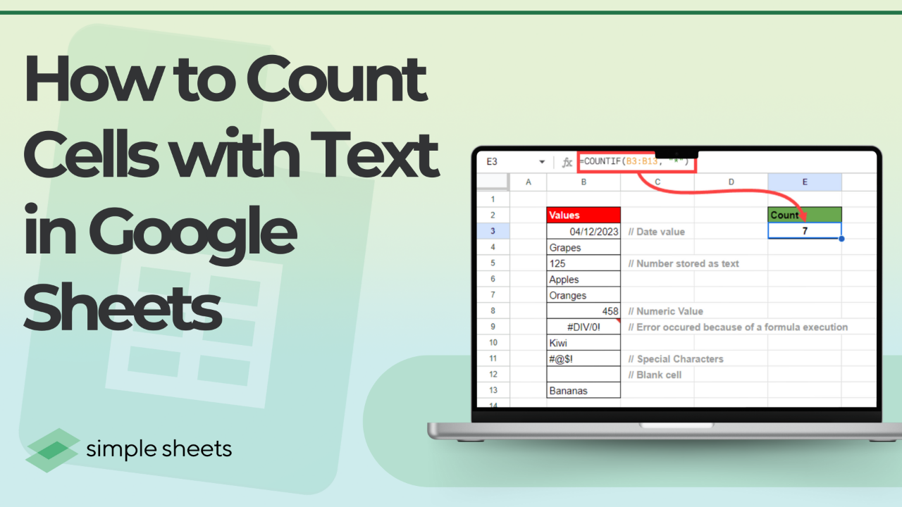
Quick answer: how to count cells with text in Google Sheets
To count cells with text in Google Sheets, use =COUNTIF(range, "*"). The asterisk wildcard matches any text string, so it counts every cell holding text and ignores numbers and blanks. Use =COUNTA(range) to count text and numbers together, =SUMPRODUCT(--ISTEXT(range)) for a strict text-only count, and =COUNTUNIQUE(range) for distinct values.
Last updated: August 18, 2026
Table of Contents
- Quick Reference: Google Sheets Count Text Formulas
- Counting Cells with Text Using COUNTIF
- COUNT vs COUNTA vs COUNTIF vs COUNTIFS vs COUNTBLANK vs COUNTUNIQUE
- Text vs Non-Text Cells: What Counts?
- Counting Non-Empty Cells with COUNTA
- Strict Text-Only Counts with SUMPRODUCT and ISTEXT
- Counting Cells That Contain Specific Text
- How Wildcards Work, and Where They Break
- Counting Text with Two or More Conditions
- Counting Text Case-Sensitively with EXACT
- Counting Unique Text Values with COUNTUNIQUE
- Counting Across Multiple Sheets
- Why Your COUNTIF Returns 0
- How to Count Cells with Text in Excel
- Frequently Asked Questions
Did you know you don't need to manually scan through rows of data to count cells with text in Google Sheets?
This is a vital skill that can save you valuable time. Google Sheets offers several built-in functions like COUNTIF and SUMPRODUCT to make this process seamless. In this guide, you'll learn multiple ways to count cells with text in Google Sheets, from the one-line COUNTIF wildcard count to multi-condition, case-sensitive and unique-value counts.
Get our free Excel formulas cheat sheet
Plus new tutorials and template drops. Enter your email and we'll send it over.

Quick Reference: Google Sheets Count Text Formulas
Use this table to find the right Google Sheets count formula for what you actually need.
| Goal | Formula | Description |
|---|---|---|
| Count any text | =COUNTIF(range, "*") |
Counts all cells with text characters (including numbers stored as text). |
| Count text (strict) | =SUMPRODUCT(--ISTEXT(range)) |
Counts only true text values, ignoring numbers formatted as text. |
| Count specific text | =COUNTIF(range, "Apple") |
Counts cells matching that word exactly, whole cell only. |
| Count partial match | =COUNTIF(range, "*Apple*") |
Counts a cell if the word appears anywhere inside it. |
| Count with two conditions | =COUNTIFS(A2:A10, "Apple", B2:B10, "Fruit") |
Counts rows only where every condition is true at once. |
| Count case-sensitively | =SUMPRODUCT(--EXACT(range, "Apple")) |
Treats "Apple" and "apple" as different values. |
| Count unique text | =COUNTUNIQUE(range) |
Counts distinct entries once each. Google Sheets only, Excel has no equivalent. |
| Count not blank | =COUNTA(range) |
Counts everything that is not empty (numbers and text). |
| Count the blanks | =COUNTBLANK(range) |
Counts empty cells, and also counts formulas that return "". |
Counting Cells with Text Using COUNTIF (the method to reach for first)
COUNTIF is the function that answers the question directly. It counts only the cells that meet a criterion, and the asterisk wildcard is a criterion that means "any run of text characters". Numbers and truly blank cells do not match it, so they drop out of the count automatically.
Formula: =COUNTIF(range, "*")
How it works:
-
range: the cells you want to search, for example A1:A10 or A:A.
-
"*": the wildcard. It matches any sequence of characters, so any text value satisfies it.
-
Numbers, dates and empty cells are excluded, which is exactly what makes this different from COUNTA.
Example:

The formula excludes the numbers and blanks.
Rule: =COUNTIF(range, "*") answers "how many cells hold text", not "how many cells hold real words". A postcode stored as text still counts. Google documents the full criteria syntax in the official COUNTIF function reference.
COUNT vs COUNTA vs COUNTIF vs COUNTIFS vs COUNTBLANK vs COUNTUNIQUE
Most counting problems in Google Sheets are not formula problems. They are function-choice problems. Six functions share the word COUNT and each counts a different thing, so picking the wrong one gives you a number that looks plausible and is wrong.
| Function | What it counts | Counts text? | Use it when |
|---|---|---|---|
COUNT |
Numbers and dates only | No | You want how many numeric entries a column holds. |
COUNTA |
Anything that is not empty | Yes, plus numbers and errors | You want how many rows were filled in at all. |
COUNTIF |
Cells meeting one condition | Yes, with a wildcard or a word | You want text only, or one specific value. |
COUNTIFS |
Cells meeting every condition | Yes, across several columns | Your condition has two or more parts. |
COUNTBLANK |
Empty cells | No, it is the inverse | You are auditing a sheet for missing entries. |
COUNTUNIQUE |
Distinct values, once each | Yes, plus numbers | You want how many different values appear, not how many rows. |
Rule: COUNT counts numbers, COUNTA counts entries, COUNTIF counts matches, COUNTUNIQUE counts distinct values. If your result is higher than you expected, you almost certainly reached for COUNTA when you wanted COUNTIF.
Text vs. Non-Text Cells: What Counts?
Before applying the formulas, you need to understand what "text" means in Google Sheets:
-
Text includes any non-numeric values, such as words, letters, and symbols.
-
Cells containing spaces or empty strings ("") from formulas may also be counted as text.
-
Numbers formatted as text will still be considered text.
-
Blank cells are not counted unless explicitly included in the function.
Counting Non-Empty Cells with COUNTA
The simplest way to count non-empty cells is the COUNTA function. However, this Google Sheets function counts cells with text and numbers, so it is not the tool when only text cells matter.
Formula: =COUNTA(range)
How it works:
-
COUNTA counts all non-blank cells in the specified range.
-
It includes both text and numbers but doesn't count blank cells.
Example:

If we use =COUNTA(A1:A5), the result will be 4 (excluding the blank cell).
Rule: COUNTA counts a formula that returns "" as filled. If a column of formulas gives you a suspiciously round COUNTA, that is why.
Strict Text-Only Counts with SUMPRODUCT and ISTEXT
For more accuracy, combine SUMPRODUCT with ISTEXT. Use it when you have mixed data types and want a strict count of text-only cells, including when numbers have been stored as text.
Formula: =SUMPRODUCT(--ISTEXT(range))
How it works:
-
ISTEXT(range): Returns TRUE for text cells and FALSE for non-text cells.
-
--ISTEXT(range): Converts TRUE to 1 and FALSE to 0.
-
SUMPRODUCT then sums up the values, giving an accurate count of text cells.
Example:

Using =SUMPRODUCT(--ISTEXT(A1:A4)), the result will be 2, as only two cells contain text.
To ignore cells that hold nothing but spaces, add a TRIM test:
=SUMPRODUCT(--(TRIM(A1:A100)<>""), --ISTEXT(A1:A100))
Counting Cells That Contain Specific Text
You can count cells containing specific text with COUNTIF. See what the formula looks like below:
Formula: =COUNTIF(range, criteria)
-
range – The data range where you want to count occurrences.
-
criteria – The text you’re looking for. Remember that this formula only counts exact matches.
Example:
Suppose you have sample data of fruits in column A (A2:A10). To count how many times "Apple" appears in column A, use:
=COUNTIF(A2:A10, "Apple")

The result is 3 since the exact match "Apple" appears thrice.
Rule: =COUNTIF(A2:A10,"Apple") counts whole-cell matches only. If you want "Green Apple" included, you need "*Apple*".
How do wildcards work in Google Sheets, and where do they break?
If you need to count cells that contain a word but may have other text as well, such as "Green Apple" or "Apple Juice", you need wildcards. This is useful for analysing customer reviews where a keyword appears in different contexts.
Wildcard symbols in Google Sheets:

| Wildcard | Meaning | Example | Matches |
|---|---|---|---|
* |
Any number of characters, including none | "*Apple*" |
Apple, Green Apple, Apple Juice |
? |
Exactly one character | "b?g" |
bag, big, bug, but not bang |
~ |
Escape, treat the next wildcard literally | "~*" |
A cell whose actual content is an asterisk |
Example:

This counts any cell that contains "Apple" as part of a longer string, like "Green Apple" or "Apple Juice".
Three gotchas cause nearly every wildcard bug:
- Wildcards do not work on numbers.
=COUNTIF(A2:A10,"*5*")will not find the numeric value 1500. Wildcards only match text, which is precisely why"*"is a reliable text-only test. - You must escape a literal asterisk or question mark. To count cells that literally contain a question mark, use
=COUNTIF(A2:A10,"*~?*"). Without the tilde, the question mark is read as "any single character" and your count balloons. - Wildcard matching is not case-sensitive.
"*apple*"and"*APPLE*"return the same number.
When wildcards are not expressive enough, Google Sheets gives you an option Excel does not have: regular expressions, through REGEXMATCH.
=SUMPRODUCT(--REGEXMATCH(A2:A100, "Apple|Pear"))
Rule: The asterisk means "any run of characters", the question mark means "exactly one", and the tilde turns either back into a plain character. Reach for REGEXMATCH only when the pattern is genuinely beyond that.
How do you count text with two or more conditions?
COUNTIF takes exactly one condition. The moment your question has an "and" in it, you need COUNTIFS, which counts only the rows where every range and criteria pair is satisfied. For instance, you can filter results on both product name and category when tracking sales data.
Example:
Suppose you have a dataset with the categories "Product" and "Category." To count only "Apple" in the "Fruit" category, use:
=COUNTIFS(A2:A10, "Apple", B2:B10, "Fruit")

The output is 3 since three Apples belong to the "Fruit" category.
Three variations worth keeping:
- Text but not blanks or spaces:
=COUNTIFS(A2:A100, "*", A2:A100, "<> ") - Text within a date window:
=COUNTIFS(A2:A100, "*", C2:C100, ">="&DATE(2026,1,1)) - Either of two words (an OR count):
=SUM(COUNTIF(A2:A100, {"*apple*","*pear*"})), because COUNTIFS cannot express OR on its own.
Rule: COUNTIFS is AND, an array constant inside COUNTIF is OR. Every range in a COUNTIFS must be the same size or Sheets returns an error.
Counting Text Case-Sensitively with EXACT
Google Sheets formulas like COUNTIF and COUNTIFS are not case-sensitive. Hence, "Apple" and "apple" are treated the same. This is a problem for case-sensitive inventory tracking, SKUs, coupon codes and case-based identifiers.
Example:
To distinguish between "Apple" and "apple," use this formula:
=SUMPRODUCT(--EXACT(A2:A7, "Apple"))

For a case-sensitive partial match, swap SEARCH (case-insensitive) for FIND (case-sensitive):
=SUMPRODUCT(--ISNUMBER(FIND("Apple", A2:A100)))
Rule: If capitalisation is meaningful in your data, COUNTIF is the wrong tool. EXACT for whole cells, FIND for partial matches.
Counting Unique Text Values with COUNTUNIQUE
Counting cells with text and counting distinct text values are different questions. A column with "Apple" five times has five text cells and one unique value.
This is where Google Sheets is genuinely easier than Excel. COUNTUNIQUE is built in and takes a range directly:
=COUNTUNIQUE(A2:A100)
COUNTUNIQUE counts numbers as well as text, and it ignores truly empty cells. To count distinct text values only, filter first:
=COUNTA(UNIQUE(FILTER(A2:A100, ISTEXT(A2:A100))))
For distinct values that also meet a condition, COUNTUNIQUEIFS works like COUNTIFS:
=COUNTUNIQUEIFS(A2:A100, B2:B100, "Fruit")
Rule: COUNTUNIQUE counts a value once no matter how many rows it fills. If your unique count is one higher than expected, an empty string from a formula is being counted as a distinct value.
How do you count cells with text across multiple sheets?
COUNTIF does not accept a 3D reference. Typing =COUNTIF(Jan:Mar!A:A,"*") returns an error, which surprises people who expect it to work like SUM.
The simplest reliable approach is to add the sheets together explicitly:
=COUNTIF(Jan!A2:A100,"*") + COUNTIF(Feb!A2:A100,"*") + COUNTIF(Mar!A2:A100,"*")
For many sheets, list the sheet names in a helper column (say E2:E13) and let INDIRECT build the references:
=SUMPRODUCT(COUNTIF(INDIRECT("'"&E2:E13&"'!A2:A100"), "*"))
Rule: INDIRECT is volatile and recalculates on every change, and it breaks if a sheet is renamed. On a large spreadsheet, plain addition is faster and safer than the clever version.
Why does your COUNTIF return 0?
A COUNTIF that returns 0 when you can plainly see matches on screen almost always comes down to one of these causes. Work through them in this order.
| Symptom | Cause | Fix |
|---|---|---|
| Returns 0 but the value is visible | Trailing or leading spaces in the data | Clean the column with TRIM, or match with "*Apple*" instead of "Apple" |
| Counting numbers returns 0 | Numbers stored as text, or text stored as numbers | Wildcards never match numeric values. Compare with =COUNT(range) to see which type you actually have |
| Undercounts by a few | Non-breaking spaces (CHAR(160)) pasted in from a web page | =TRIM(SUBSTITUTE(A1,CHAR(160)," ")) |
| Mismatched ranges error | COUNTIFS ranges are different sizes | Make every range in the COUNTIFS span identical rows |
| Counts blank-looking cells | Formulas returning "" or cells holding a single space | Add a second condition: =COUNTIFS(A2:A100,"*",A2:A100,"<> ") |
| Result never changes | The range is hard-coded and new rows fall outside it | Use a whole-column reference such as A2:A instead of A2:A100 |
Rule: A COUNTIF that returns 0 is a data problem, not a formula problem, about nine times out of ten. Test with =COUNTIF(A:A,"*Apple*") first. If the wildcard version finds them, you have stray spaces.
How to Count Cells with Text in Excel
The core formula is identical in Excel: =COUNTIF(range, "*") behaves the same way in both applications. The differences appear in the advanced cases. Excel has no COUNTUNIQUE, so distinct counts need =COUNTA(UNIQUE(range)) or a reciprocal-COUNTIF pattern on older versions, and Excel has no REGEXMATCH for criteria. For the Excel versions of everything on this page, see our full guide to how to count cells with text in Excel.
Final Thoughts
Counting cells with text in Google Sheets comes down to picking the right function before you write anything. COUNTIF with a wildcard handles most cases, COUNTIFS handles conditions, COUNTUNIQUE handles distinct values, and SUMPRODUCT handles everything COUNTIF cannot. Reach for the advanced patterns only when the simple ones give you a number you do not trust.

For more easy-to-follow Excel guides and the latest Excel Templates, visit Simple Sheets and the related articles section of this blog post.
Subscribe to Simple Sheets on YouTube for the most straightforward Excel video tutorials!
Frequently Asked Questions
1. How do I count cells with text in Google Sheets?
Use =COUNTIF(range, "*"). The asterisk wildcard matches any text string, so the formula counts every cell holding text and skips numbers, dates and blank cells. For a strict count that also excludes numbers stored as text, use =SUMPRODUCT(--ISTEXT(range)).
2. Can I count only unique text values in Google Sheets?
Yes. Google Sheets has a built-in function for this: =COUNTUNIQUE(A2:A10) counts each distinct value once. To restrict it to text only, use =COUNTA(UNIQUE(FILTER(A2:A10, ISTEXT(A2:A10)))), and for distinct values that also meet a condition use COUNTUNIQUEIFS.
3. Why is my COUNTIF formula not working correctly?
Check that your criteria use the correct syntax, especially for partial text, where you need wildcards such as =COUNTIF(A2:A10, "*Apple*"). Also make sure your data does not contain trailing spaces, non-breaking spaces pasted from a web page, or numbers stored as text.
4. How do I count case-sensitive text in Google Sheets?
Use SUMPRODUCT with EXACT, as in =SUMPRODUCT(--EXACT(A2:A10, "Apple")), to distinguish between uppercase and lowercase entries. This treats "Apple" and "apple" as different values. For a case-sensitive partial match, use =SUMPRODUCT(--ISNUMBER(FIND("Apple", A2:A10))).
5. What is the difference between COUNTA and COUNTIF in Google Sheets?
COUNTA counts every cell that is not empty, including numbers, errors and formulas that return an empty string. COUNTIF counts only the cells matching a criterion, so =COUNTIF(range, "*") counts text and leaves numbers out. Use COUNTA for "how many rows were filled in" and COUNTIF for "how many hold text".
6. How do I count cells with text and two conditions?
Use COUNTIFS, which counts a row only when every range and criteria pair is true. For example =COUNTIFS(A2:A10, "Apple", B2:B10, "Fruit"). Every range in a COUNTIFS must span the same number of rows, otherwise Google Sheets returns an error.
7. Can COUNTIF count across multiple sheets in Google Sheets?
Not with a 3D reference. =COUNTIF(Jan:Mar!A:A,"*") returns an error. Add the sheets explicitly with =COUNTIF(Jan!A2:A100,"*") + COUNTIF(Feb!A2:A100,"*"), or use =SUMPRODUCT(COUNTIF(INDIRECT("'"&SheetList&"'!A2:A100"),"*")) where SheetList holds the sheet names.
8. How do I count cells that do not contain certain text?
Google Sheets has no "does not contain" wildcard criterion, so subtract instead: =COUNTIF(A2:A10,"*") - COUNTIF(A2:A10,"*Apple*"). For an exact non-match rather than a partial one, =COUNTIF(A2:A10,"<>Apple") works directly.
Get our free Excel formulas cheat sheet
Plus new tutorials and template drops. Enter your email and we'll send it over.
Related Articles
How to Count Cells with Text in Excel
How to Enter New Line in a Cell in Google Sheets
Want to Make Excel Work for You? Try out 5 Amazing Excel Templates & 5 Unique Lessons
We hate SPAM. We will never sell your information, for any reason.