How to Use SUMPRODUCT with Multiple Criteria in Excel
Feb 06, 2023
Quick answer
SUMPRODUCT multiplies the matching entries of two or more arrays and then adds up the results. To apply multiple criteria, wrap each condition in brackets and multiply them by the values you want summed, like =SUMPRODUCT((A2:A8="Monday")*(B1:F1="Vince")*B2:F8). Multiplying conditions means AND. Adding them with a plus sign means OR.
Do you have data in multiple columns you need to add up, but only when specific criteria are met? Do you have a tough time making Excel formulas do the work for you?
If so, a SUMPRODUCT with multiple criteria is a great solution to simplify your data crunching.
Get our free Excel formulas cheat sheet
Plus new tutorials and template drops. Enter your email and we'll send it over.
What this guide covers
- What is the SUMPRODUCT function?
- What is the SUMPRODUCT formula for multiple criteria?
- How do you sum the product of two columns?
- How to build a SUMPRODUCT with multiple criteria, step by step
- How do you use OR logic in SUMPRODUCT?
- SUMPRODUCT vs SUMIFS: which should you use?
- Can you use IF inside SUMPRODUCT?
- How to highlight the matching value with conditional formatting
- Why is your SUMPRODUCT formula not working?
- Frequently asked questions
Read Also: Excel Repeat Last Action: What is it and How Does it Work?

What is the SUMPRODUCT function?
The SUMPRODUCT function in Excel multiplies the matching entries of two or more arrays and then adds up all of those products. The multiplication happens first, row by row, and the sum happens last. That second half is the part people forget, and it is the reason SUMPRODUCT returns one number rather than a column of numbers.
The rule to remember: SUMPRODUCT is not a multiply function. It is a multiply-then-add function, and the addition is what makes it useful for criteria work.
Because a comparison like A2:A8="Monday" produces an array of TRUE and FALSE values, and because TRUE behaves as 1 and FALSE behaves as 0 in arithmetic, multiplying your values by those comparisons zeroes out every row that fails the test. Everything that survives gets summed. That single behaviour is what lets one function handle several conditions at once.
| Argument | Required? | What it does |
|---|---|---|
| array1 | Required | The first range or array whose components are multiplied and then added. |
| [array2], [array3]... | Optional | Array arguments 2 to 255. SUMPRODUCT accepts up to 255 arrays in total. |
Syntax: =SUMPRODUCT(array1, [array2], [array3], ...). Microsoft documents the full argument list and the error behaviour in the official SUMPRODUCT function reference.
Two behaviours are worth knowing before you start. When arrays are separated by commas they must have identical dimensions, or Excel returns #VALUE!. And SUMPRODUCT treats non-numeric entries, including text and blanks, as zeros rather than throwing an error, which is why a bad formula here often returns a quietly wrong number instead of a visible error.
What is the SUMPRODUCT formula for multiple criteria?
The multiple-criteria pattern replaces the commas with multiplication signs. That is the whole trick, and it is a supported use of the function rather than a workaround.
Multiple criteria (AND logic):
=SUMPRODUCT((criteria range 1=criterion 1)*(criteria range 2=criterion 2)*value range)
Counting rows that meet one condition:
=SUMPRODUCT((C2:C10<B2:B10)*1)
That second formula does not sum anything from your data. It compares column C against column B row by row and returns a count of the rows where C is smaller. The *1 converts the TRUE and FALSE results into 1s and 0s so they can be added. Use it when you want a count under conditions that COUNTIFS cannot express, such as comparing two columns against each other.
The rule to remember: multiply your criteria together to mean AND, and put the range you want totalled last.
SUMPRODUCT accepts up to 255 array arguments, so in practice the number of criteria you can stack is limited by readability, not by Excel.
Read Also: Excel Macro Button: What is it and How to Create One
How do you sum the product of two columns?
This is the original job SUMPRODUCT was built for, and it needs no criteria at all. If column B holds quantities in B2:B10 and column C holds unit prices in C2:C10, the order total is:
=SUMPRODUCT(B2:B10, C2:C10)
Excel multiplies B2 by C2, B3 by C3 and so on down the two ranges, then adds every one of those results into a single figure. It replaces a helper column of line totals plus a SUM at the bottom. If you later need to restrict that total to one region or one month, you add a criteria bracket to the same formula rather than rebuilding it, which is covered in the walkthrough below.
The rule to remember: commas between ranges means straight multiply-and-add, and those ranges must be exactly the same size.
How to build a SUMPRODUCT with multiple criteria, step by step
This walkthrough uses a grid: days listed down column A, names listed across row 1, and the numbers you want to total sitting in the block B2:F8. The goal is a two-way lookup, matching one name across the columns and one day down the rows, and totalling only the cell where they intersect.
- Prepare your data.
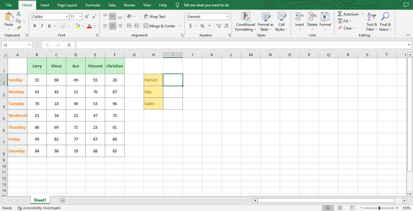
- The block of numbers in B2:F8 is the range of values you want totalled.
- The first column, A2:A8, holds the list of Days.
- The first row, B1:F1, holds the list of Names.
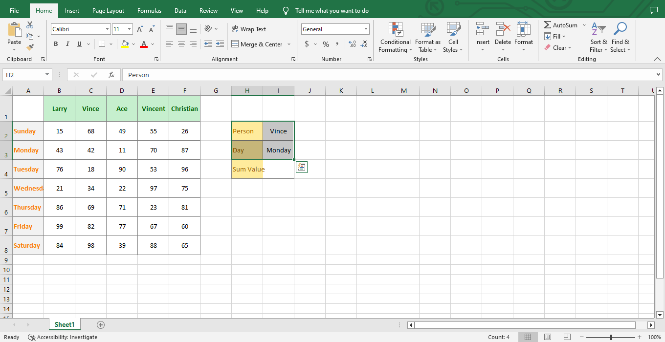
- Set up your two criteria cells. Put the name you want in cell I2 and the day you want in cell I3. Pointing the formula at cells rather than typing the criteria inside it means you can change the answer later without editing the formula.
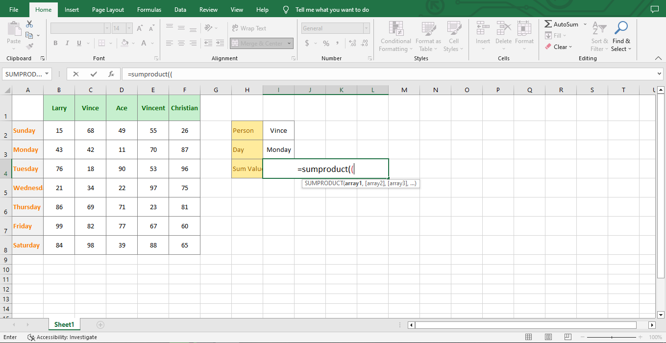
- Start the formula in cell I4. Type =SUMPRODUCT( and leave the bracket open. The completed formula for this example is =SUMPRODUCT(B2:F8*(B1:F1=I2)*(A2:A8=I3)), and the next four steps build it one piece at a time.
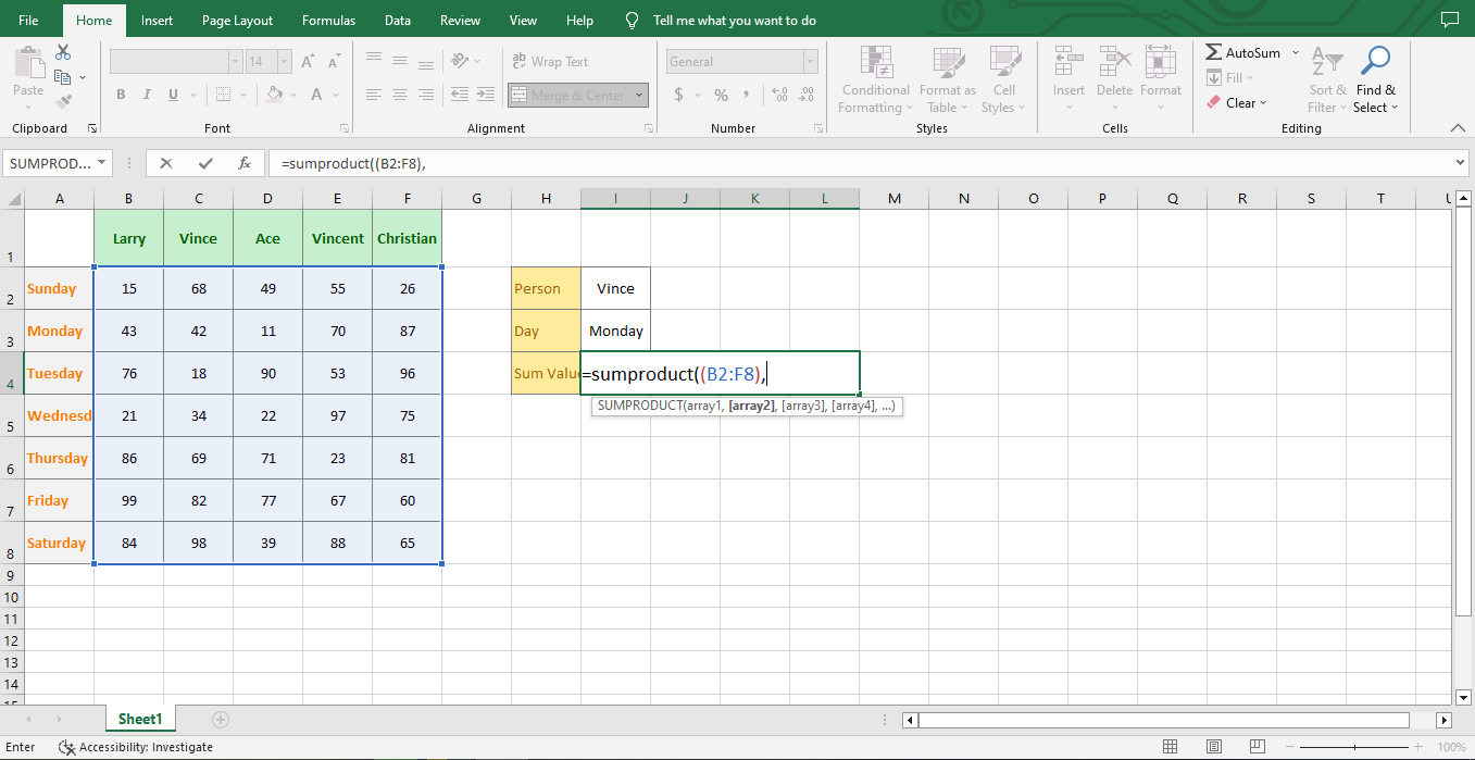
- Select the block of numbers B2:F8. This is the value range. You can drag across it or type the reference by hand.
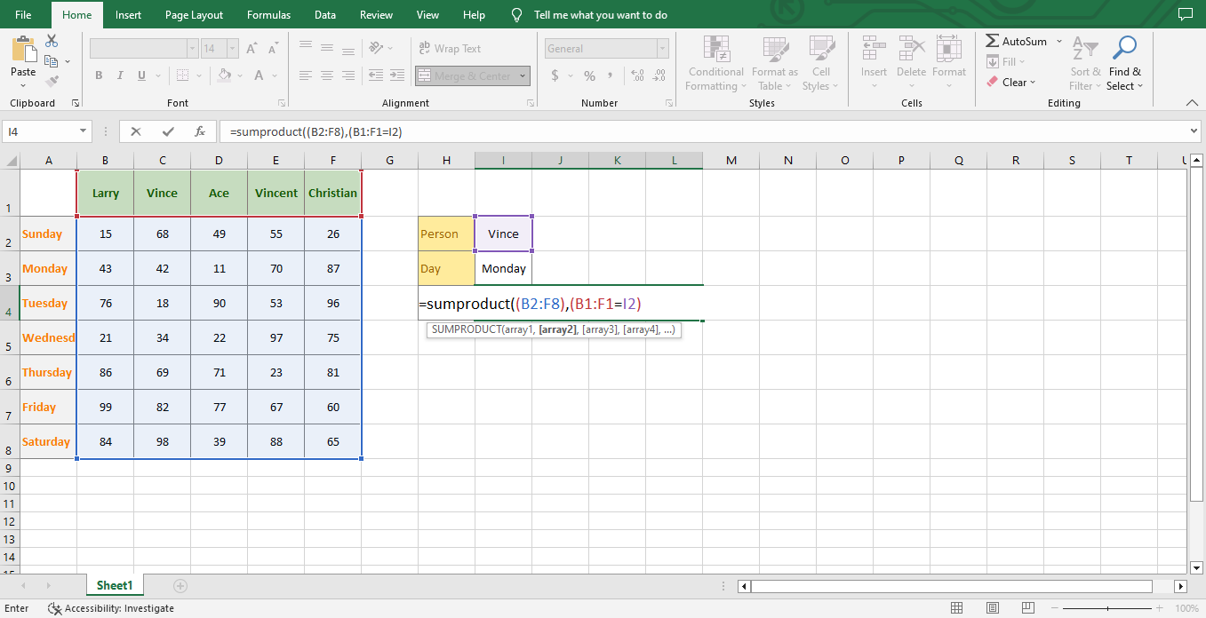
- Add the first condition. Type an asterisk, open a bracket, select the name row B1:F1, type an equals sign and click cell I2 which holds "Vince", then close the bracket. You now have *(B1:F1=I2).
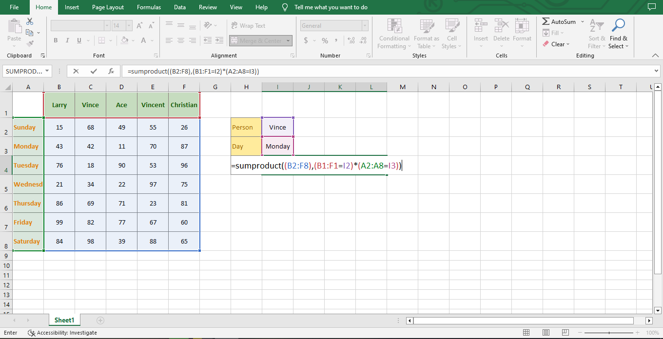
- Add the second condition. Type another asterisk, open a bracket, select the day column A2:A8, type an equals sign and click cell I3 which holds "Monday", then close the bracket. The asterisk between the two conditions is what makes this an AND test.
- Close the formula and press Enter. The result is 42.
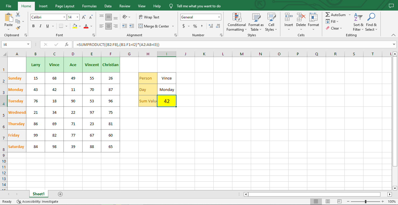
Why the different shapes still work. B1:F1 is one row wide, A2:A8 is one column tall, and B2:F8 is the rectangle between them. When you multiply a row array by a column array with the asterisk operator, Excel expands both to cover the full rectangle, so all three end up the same size. This is the one situation where SUMPRODUCT arrays do not have to start out with matching dimensions, and it is exactly what makes a two-way lookup possible.
How do you use OR logic in SUMPRODUCT?
Swap the multiplication sign for a plus sign. Multiplying conditions asks for rows that satisfy every test. Adding them asks for rows that satisfy at least one.
To total sales for either the North region or the South region:
=SUMPRODUCT(((A2:A100="North")+(A2:A100="South"))*B2:B100)
The extra pair of brackets around the added conditions matters. Without them Excel applies the multiplication before the addition and the answer is wrong rather than broken, which is the hardest kind of mistake to spot.
The rule to remember: asterisk means AND, plus means OR, and OR conditions must be wrapped in their own bracket before you multiply by the value range.
One caution on OR logic. If a row can satisfy two of your OR conditions at once, the addition produces a 2 rather than a 1 and that row gets counted twice. Wrapping the whole thing in a greater-than test fixes it: =SUMPRODUCT((((A2:A100="North")+(B2:B100="Priority"))>0)*C2:C100).
SUMPRODUCT vs SUMIFS: which should you use?
SUMIFS is the simpler tool and it should be your default for straightforward multi-criteria sums. SUMPRODUCT earns its place when SUMIFS cannot express the question.
| The job | Use SUMIFS | Use SUMPRODUCT |
|---|---|---|
| Sum one column where two other columns match fixed criteria | Yes, shorter and faster | Works, but longer |
| Criteria running across a row as well as down a column (two-way lookup) | No | Yes |
| Compare two columns against each other, such as actual below budget | No | Yes |
| Multiply two columns together before summing, such as quantity by price | No | Yes |
| OR logic across different columns | No, needs several SUMIFS added together | Yes, with the plus operator |
| Apply a function such as MONTH or LEFT to the criteria range | No | Yes |
| Sum a whole column reference like A:A | Yes, handles it efficiently | Avoid, it forces a very large calculation |
The rule to remember: reach for SUMIFS first, and switch to SUMPRODUCT the moment your criteria involve a calculation, a row-and-column intersection, or a comparison between two ranges.
Can you use IF inside SUMPRODUCT?
You can, but in almost every case you should not. SUMPRODUCT already handles conditions natively through its arithmetic, so an IF inside it is redundant and makes the formula slower and harder to read.
These two return the same answer:
=SUMPRODUCT(IF(A2:A100="North", B2:B100, 0))
=SUMPRODUCT((A2:A100="North")*B2:B100)
The second is the one to use. It is shorter, and in versions of Excel before 2021 the IF version had to be confirmed as an array formula with Ctrl+Shift+Enter while the multiplication version never did.
There is one case where IF genuinely helps. If your value range can contain text or error values that would poison the arithmetic, IFERROR or IF can clean the range first. Otherwise, express the condition with a comparison and let the multiplication do the work.
Read Also: Excel COUNTIF Function: Simple Guide For Beginners
How to highlight the matching value with conditional formatting
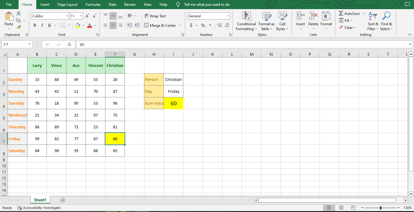
Using conditional formatting in Excel, you can highlight the cell in your grid that matches the total SUMPRODUCT returned. It turns the answer into something you can see on the sheet rather than a number sitting off to the side.
- Select the block of numbers.
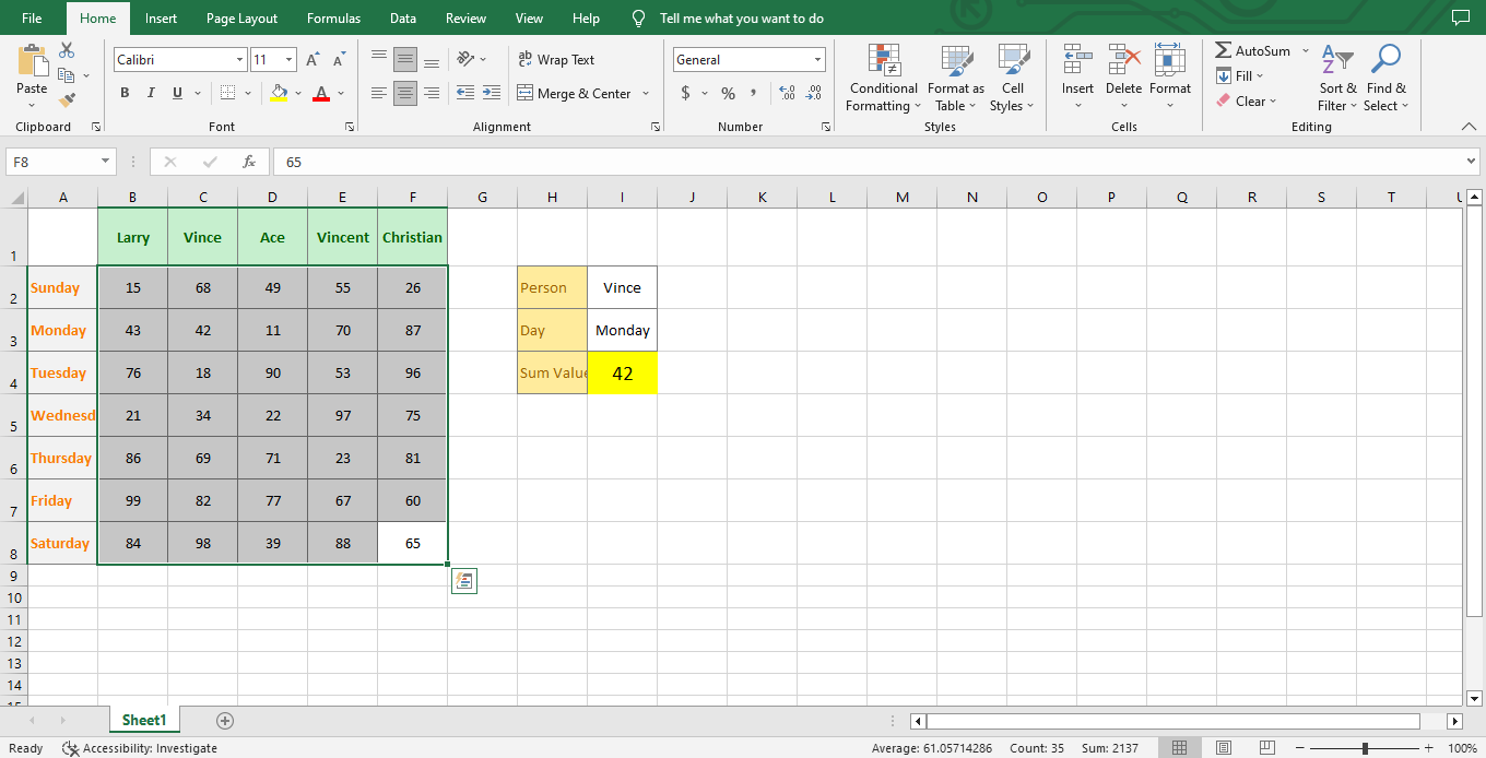
- Open Conditional Formatting on the Home tab and click New Rule.
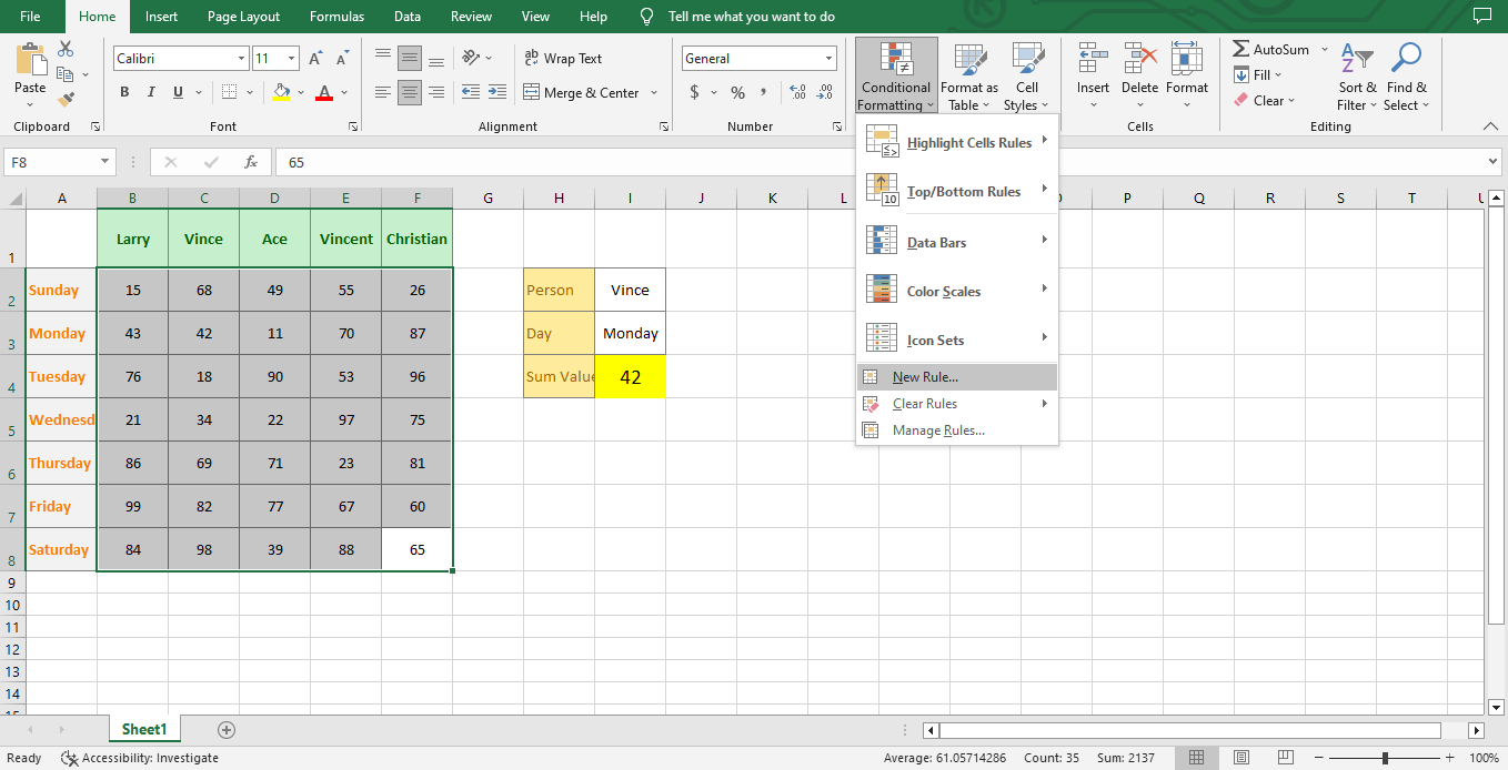
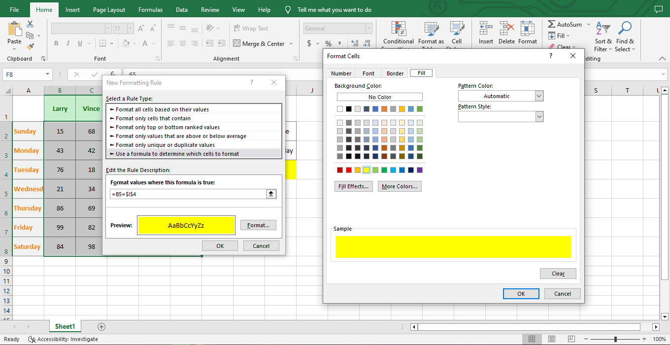
- Choose "Use a formula to determine which cells to format" and enter =B5=$I$4, then pick a fill colour under Format and click OK. Write the formula against the top-left cell of your selection and lock the answer cell with dollar signs, so the rule tests every cell in the block against the one result.
- Change the name or the day in your criteria cells and both the total and the highlight follow, with no need to retype the SUMPRODUCT formula.
Where to find SUMPRODUCT in the ribbon
- Go to the "Formulas" tab in Microsoft Excel.
- Click Math & Trig and select SUMPRODUCT from the list.
Why is your SUMPRODUCT formula not working?
SUMPRODUCT fails in a small number of predictable ways. Work down this table before rewriting the formula.
| What you see | Likely cause | Fix |
|---|---|---|
| #VALUE! | Comma-separated arrays are different sizes, for example C2:C10 against D2:D5 | Make every range the same height and width. Count the rows, not the labels. |
| #VALUE! with ranges that look identical | One range contains a cell holding an error value such as #N/A | Clean the source data, or wrap the range in IFERROR. Microsoft covers this case in its #VALUE! in SUMPRODUCT guide. |
| Returns 0 with no error | Criteria text does not match exactly, usually a trailing space or a number stored as text | Test one condition on its own first. Use TRIM on the source, and check that "42" is a number and not text. |
| Returns a count instead of a total | You multiplied the conditions but forgot to multiply by the value range | Add the value range as the last item, or keep the *1 if a count is what you wanted. |
| Answer is roughly double what you expect | OR conditions added together, and some rows satisfy more than one | Wrap the added conditions in a greater-than-zero test. |
| Workbook is slow to calculate | Whole-column references such as A:A inside SUMPRODUCT | Limit ranges to the rows you actually use, or convert the data to an Excel Table and use structured references. |
| A missing or misplaced bracket breaks the formula | Each condition needs its own pair of brackets | Count opening and closing brackets. Excel colour-codes matching pairs as you type. |
Final thoughts on using SUMPRODUCT with multiple criteria in Excel
SUMPRODUCT is worth learning properly because it answers questions the simpler summing functions cannot reach: totals that depend on a row and a column at the same time, comparisons between two columns, and any sum that needs a multiplication before it is added.
Start with the two-column version, add one criteria bracket, then a second. Try each pattern above on your own data and see which fits, and don't forget to check out the rest of the Simple Sheets blog for more how-to and step-by-step guides.
Frequently asked questions about SUMPRODUCT with multiple criteria in Excel
What is the SUMPRODUCT function in Excel?
SUMPRODUCT multiplies the matching entries of two or more arrays and then adds all of those products into a single result. It is a multiply-then-add function, which is why =SUMPRODUCT(B2:B10, C2:C10) returns one order total rather than a column of line totals.
How do you use SUMPRODUCT with multiple criteria?
Wrap each condition in its own bracket, multiply the conditions together, and put the range you want summed last. For example =SUMPRODUCT((A2:A100="North")*(B2:B100="March")*C2:C100) totals column C only for rows that are both North and March.
Can you use IF inside SUMPRODUCT?
You can, but it is usually unnecessary. SUMPRODUCT handles conditions through arithmetic, so =SUMPRODUCT((A2:A100="North")*B2:B100) is shorter and faster than the IF version and never needed Ctrl+Shift+Enter in older versions of Excel.
What is the difference between SUMPRODUCT and SUMIFS?
SUMIFS is simpler and faster for plain multi-criteria sums. SUMPRODUCT is the one to use when criteria run across a row as well as down a column, when you need to compare two columns against each other, or when values must be multiplied before they are summed.
Why does my SUMPRODUCT formula return #VALUE!?
Almost always because comma-separated arrays are different sizes, or because one of the ranges contains an error value. Make every range the same height and width, and clean or wrap any range that holds #N/A or similar errors.
How many arrays can SUMPRODUCT handle?
Microsoft documents SUMPRODUCT as accepting array1 plus array arguments 2 to 255, so 255 arrays in total. In practice readability limits you long before Excel does.

Related Articles:
SUM Index-Match: What is it, and How do I use it?
How to Count Cells With Text in Excel
Greater Than or Equal To in Excel
Microsoft Excel Certification: How to Become a Professional
How to Delete Sheets in Excel: Deleting Multiple Sheets at Once
Last updated: August 21, 2026
Want to Make Excel Work for You? Try out 5 Amazing Excel Templates & 5 Unique Lessons
We hate SPAM. We will never sell your information, for any reason.