
Using Conditional Formatting in Excel
Jan 24, 2022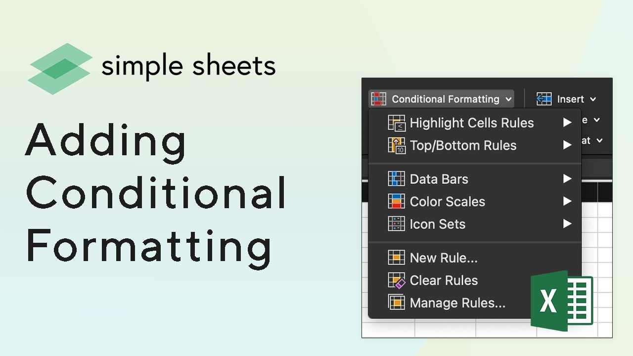
At some point, we will all encounter spreadsheets that are probably too big for Microsoft Excel. This makes looking for significant values or outliers challenging unless you’re Peter Parker with his Spidey Sense. We might not have genetically mutated spiders, but we have conditional formatting. Like charts and sparklines, conditional formatting provides another way to visualize data and make worksheets easier to understand.
Get our free Excel formulas cheat sheet
Plus new tutorials and template drops. Enter your email and we'll send it over.
Understanding Conditional Formatting Excel
Conditional formatting allows you to automatically apply formatting such as colors, icons, and data bars to one or more cells based on the cell's value. To do this, you will need to create a conditional formatting rule. For example, one of the conditional formatting rules might be: If the value is less than $2000, the cell colors are in red. Applying this rule will show cells containing values under $2000. 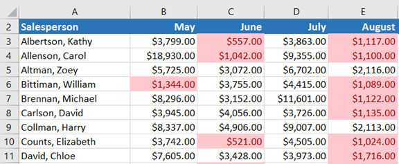
How To Create a Conditional Formatting Rule:
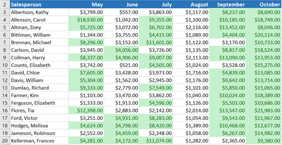
We have a worksheet with sales data in our example, and we'd like to see which salespeople are meeting their monthly sales goals. The sales target is $4000 per month, so we'll create a conditional format rule for any cells with a value above 4000.
- Select the cells required for the conditional formatting rule.
- On the Home tab, click the Conditional Formatting command. A drop-down menu will appear.
-
Hover over the desired conditional formatting type, then select or click the conditional formatting rule that you want from the list that appears. In our example, we want to highlight cells that are over $4000.

- The dialog box appears. Enter the desired value(s) in the empty field. In our example, we'll enter 4000 as our values.
- Select a formatting style from the drop-down list. For example, we'll choose Green Fill with Dark Green Text in our sample and click OK.

- Conditional formatting will be applied to the selected cells. So, our example makes it easy to see which salespeople hit the $4,000 monthly sales target.
You can apply multiple conditional formatting rules to a range of cells or a worksheet, allowing you to visualize different indicators and patterns in your data. And you can use them to format cell dialog boxes, create a new rule, or use conditional formatting to highlight or format values.
Aside from using the formatting rule dialog box to create a new conditional formatting rule, create conditions on cell values to highlight cells - using the conditional formatting rules manager or conditional formatting formula. You can also purchase pre-made models provided by simple sheets. 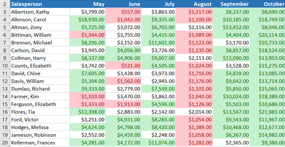
 Conditional Preformat
Excel has many predefined styles or presets, which you can use to apply conditional formatting to your data quickly. They are grouped into three categories:
- Data bars are horizontal bars added to each cell, much like a bar graph.

- Hue allows changing the color of each cell based on its value. Each color scale uses a shade of two or three colors. You can paste conditional formatting rules that apply to selected cells, like showing duplicate values that conditionally format cells rules with one or two conditional formatting rules like click highlight cells rules. For example, in the green-yellow-red color scale, the highest values are green, the middle values are yellow, and the lowest are red.

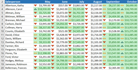
- Icon sets add a specific icon to each cell based on its value.

Using a preset conditional format:
- Select the cells required for the conditional formatting rule.

- Click the conditional formatting command. A drop-down menu will appear.
- Hover over the setting you selected earlier, then choose a setting style from the menu that appears.
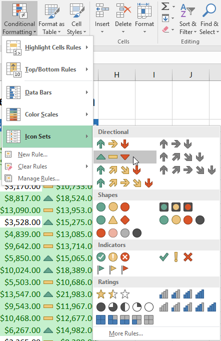
- Conditional formatting will be applied to the selected cells.
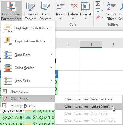
 Removing conditional formatting To remove conditional formatting:
- Click the conditional formatting command. A drop-down menu will appear.
- Hover over Clear Rules, and choose the rules you want to clear. In this example, we'll select Clear Rules from the Entire Sheet to remove all conditional formatting from the worksheet.
- Conditional formatting will be removed.

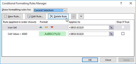
Click Manage Rules (from conditional formatting rules manager) to edit or delete specific rules. This is especially useful if you apply multiple rules to the worksheet.
 Conditional Formatting allows you to step up your spreadsheet game, not only aesthetically but also increases your spreadsheets’ functionality making your data more readable and, therefore, more helpful.
Like selecting values from column b or d etc., to apply conditional formatting based on values, contents, or absolute reference of cell values from your rule description to format corresponding cells like maximum values, click format, relative reference to other cells, or specific cells - you can easily manage rules or styles group.
If you want some great examples of conditional formatting, check out Simple Sheets’ great Excel templates, such as the Fishbone Diagram, COVID-19 Business Health Tracker, and the Excel 2022 Calendar Template! 
Want to Make Excel Work for You? Try out 5 Amazing Excel Templates & 5 Unique Lessons
We hate SPAM. We will never sell your information, for any reason.

