How to Merge Cells in Excel Without Losing Data

If you’ve ever clicked the Merge & Center button in Excel, you’ve likely seen the dreaded warning:

"Merging cells only keeps the upper-left value and discards other values."

It is a frustrating moment. You have data in three different cells that you want to bring together. However, Excel’s default setting treats your data like it’s disposable, deleting everything except the very first piece of information.

The good news? You don’t have to choose between a clean layout and keeping your data.

Whether you are trying to combine First and Last names or simply create a clean header without breaking your spreadsheet, there are several ways to get the job done.

In this guide, we’ll show you exactly how to merge cells while keeping every bit of your text intact.

• Combine the data first using TEXTJOIN, Flash Fill, Power Query, or VBA

• Check the result carefully on a few rows

• Copy → Paste Values to lock the final text

• Delete original columns only after confirming the result

• Use Center Across Selection if you only need a visual merge

• Keep a backup of the file, especially when using macros

Method 1: Using TEXTJOIN

This is the safest and most recommended method. You don’t merge cells first. Instead, you combine the contents into a new cell, then merge cells afterward only for appearance. This method works because Excel keeps all the data before any merge happens.

Let's assume this is your table:

Step 1: Add a helper column

Insert a new empty column where you want the combined result.

Step 2: Enter the formula

In the helper cell (e.g. C1), type: =TEXTJOIN(", ", TRUE, A1:B1)

What this does:

• " " → adds a space between values

• TRUE → ignores empty cells

• A1:B1 → the cells being combined

Step 3: Fill down

Drag the formula down to apply it to other rows.

Step 4: Lock the result

Right now, the result depends on the original cells. To make it permanent:

1. Select the helper column

2. Copy

3. Paste → Values only

Step 5: Remove old columns and merge visually

To improve the formatting:

1. Delete the original columns (A–C)

2. Select the remaining cells

3. Use Merge Cells or Center Across Selection

Method 2: Use Flash Fill to merge cells automatically

Flash Fill is a fast method that requires no formula. Excel examines a pattern you type once and then fills in the rest for you. This method is great when the data is simple and the pattern is clear.

Assume this is the data:

Step 1: Create a new column

Insert an empty column next to your data.

Step 2: Manually type the first result

In the first cell of the new column, type:

Step 3: Activate Flash Fill

Select the next cell below. Press Ctrl + E. Excel automatically fills the column:

Step 4: Lock the results (important)

Flash Fill creates values, not formulas. However, it’s still best practice to:

1. Select the filled column

2. Copy

3. Paste → Values only

This guarantees that nothing changes later.

Using Flash Fill with more complex data

Flash Fill can also:

• Add commas or dashes

• Reorder text (Last name, First name)

• Combine text and numbers

• Extract parts of a cell before merging

Limitations you should know

Take note:

• Since it uses no formulas, it isn't dynamic

• Can fail if data patterns vary

• Large datasets may need re-triggering

• Doesn’t work well with inconsistent spacing or typos

Method 3: Use Fill → Justify to Merge text Vertically

Fill → Justify is a feature in Microsoft Excel that lets you merge multiple cells in the same column into one cell. It only works vertically.

Assume the data in column A:

Step 1: Select the full range

Select from the first text cell down to the last cell.

Step 2: Expand the column

Expand the column to ensure the first cell can contain the combined data from all the cells.

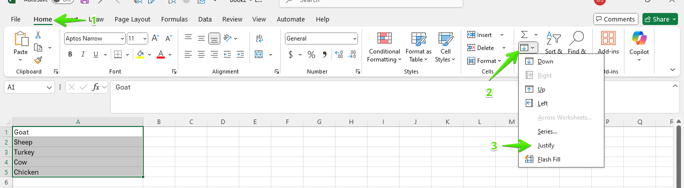
Step 3: Apply Justify

1. Go to Home

2. Click Fill

3. Choose Justify

Result:

Excel combines everything into the top cell and clears all cells below it.

Limitations you should know

Take note:

• Works only vertically

• Text only (numbers may behave unpredictably)

• No control over separators (Excel uses spaces)

• One-time action (not dynamic)

Method 4: Use Power Query to Merge Cells

Power Query is Excel’s data-cleaning and transformation tool. It’s ideal when you’re working with large datasets or when you need to repeat the same merge process regularly. Unlike normal merging, Power Query never deletes your original data.

 Sample data:

Step 1: Convert data to a table

1. Select your data

2. Press Ctrl + T

3. Click OK

Step 2: Load data into Power Query

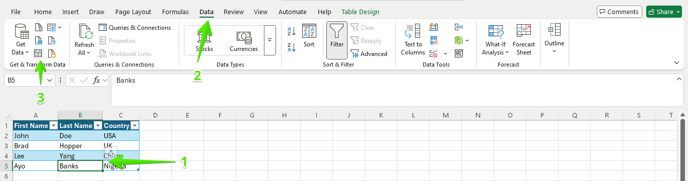
1. Click anywhere inside the table

2. Go to Data → From Table/Range

3. Power Query Editor opens

Step 3: Merge the columns

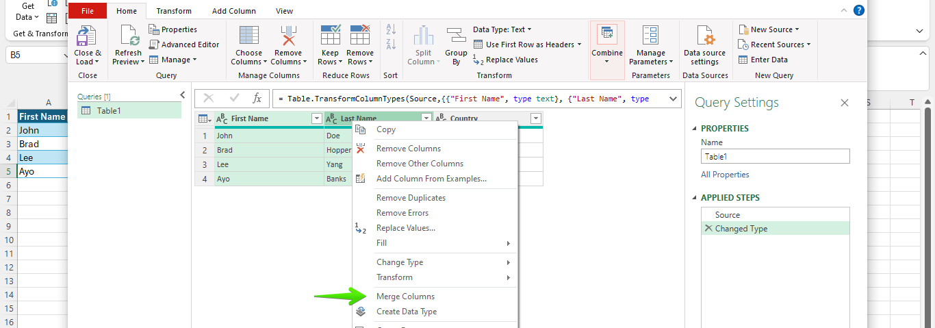
1. Hold Ctrl and select the columns you want to combine

2. Right-click → Merge Columns

3. Choose a separator (space, comma, dash, custom)

4. Name the new column

5. Click OK

Step 4: Load the result back to Excel

1. Click Close & Load

2. Excel creates a new sheet with the merged results

Best Practices for Keeping Your Data Safe

Merging cells in Excel doesn’t have to be risky. The key is following a few simple habits that prevent accidental data loss, broken formulas, and layout problems. These best practices apply regardless of the method you use.

1. Always combine data first: Use formulas, Flash Fill, Power Query, or Justify to combine content into a single cell before merging anything.

2. Use helper columns:They give you control and a safety net. You can always delete them after pasting values.

3. Paste values before deleting source data: This is the most important rule. It locks your results and prevents accidental loss.

4. Use “Center Across Selection” for appearance: If you only want a merged look, this option keeps cells separate and avoids all merge-related issues.

5. Work on a copy of the file: Especially when using Power Query. One duplicate file can save a lot of stress.

6. Test on a few rows first: Before applying any method to the full dataset, test it on 3–5 rows to confirm the results look correct.

Final Thoughts

Merging cells in Excel is safe as long as you do it in the right order. Most data loss happens when cells are merged too early. The better approach is to combine the content first, then merge it only for layout if necessary.

Whether you use formulas, Flash Fill, Power Query, or Justify, the goal is the same: keep every value intact before changing how the sheet looks.