Learn About Google Sheets Conditional Formatting Based on Another Cell

google sheets Feb 17, 2023

learn-google-sheets-conditional-formatting-based-on-another-cell

Learning about Google Sheets conditional formatting based on another cell will help you to improve your Google Sheets skillset and take your work to the next level.

In this blog, we will cover the following:

How to highlight cells using conditional formatting based on another cell value in Google Sheets.
How to use Google Sheets conditional formatting based on another cell's value.
How to use Google Sheets conditional formatting if another cell contains the text.

How to Highlight Cells Using Conditional Formatting Based on Another Cells Value

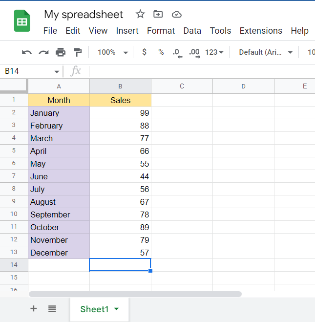
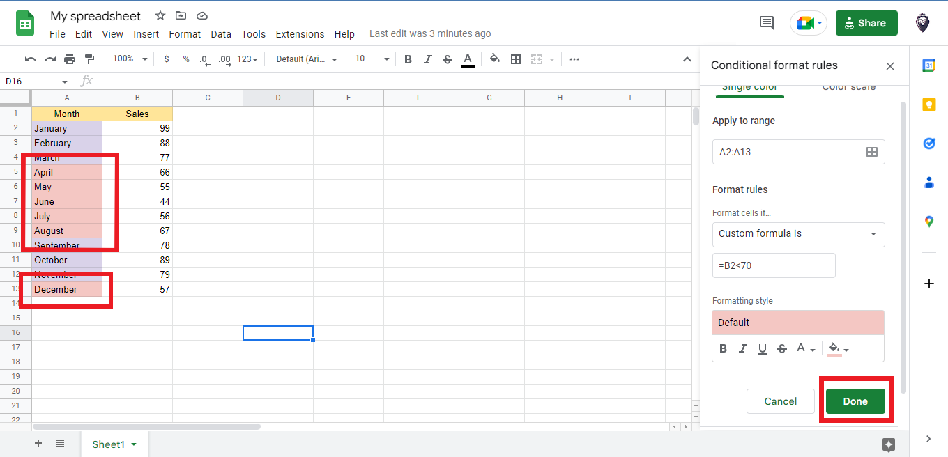
Let's assume the image below is your data:

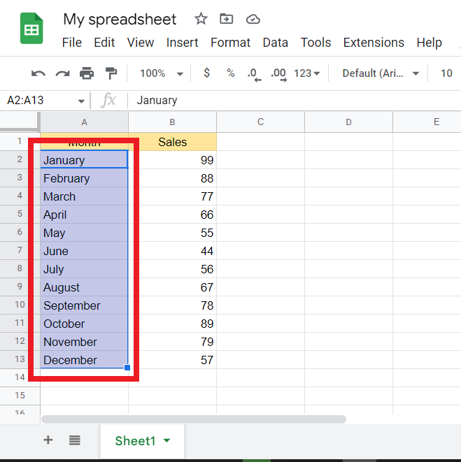
Here are the steps to use Google Sheets conditional formatting to highlight cells with months based on the number of sales:

Select the cells that contain the months.

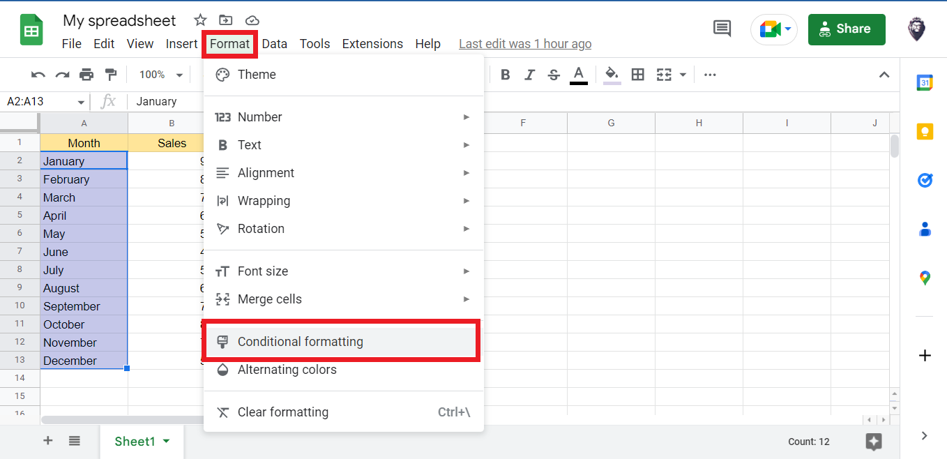
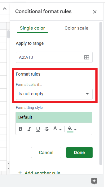
Look for the Format Tab and select Conditional Formatting.

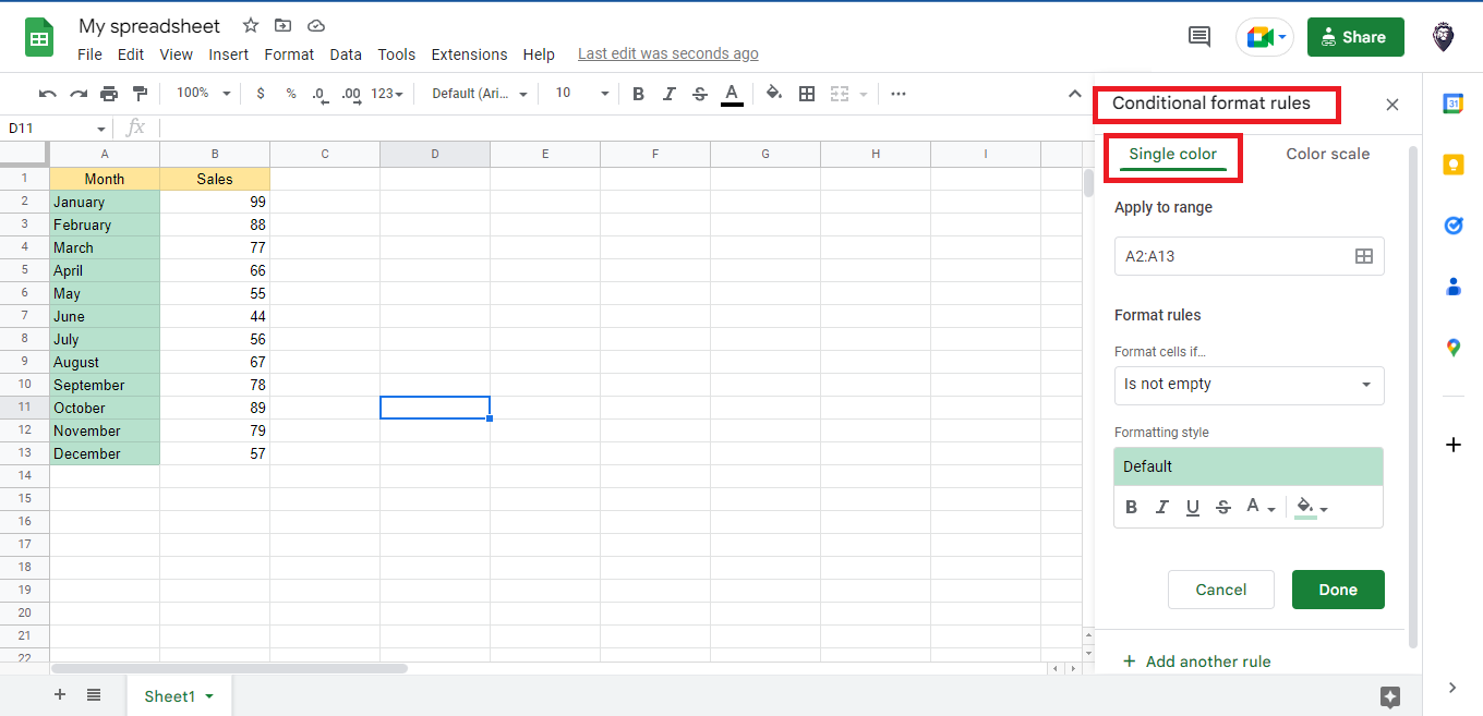
In the Conditional Formatting rules pane, select the option for Single Color.

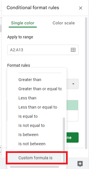
Click 'Custom Formula is' from the 'Format Cells if' drop-down menu.

In the Value field under the Format Rules, enter the value/formula: =B2<70.

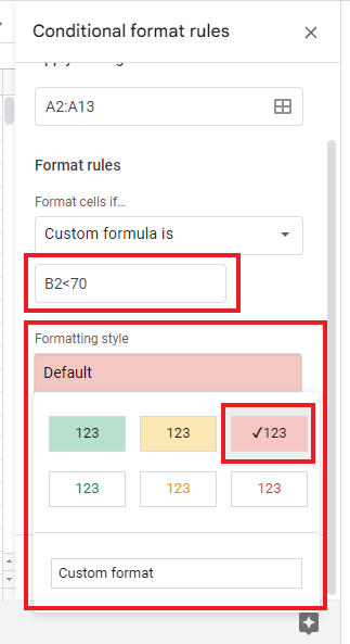
Click "Done," and Google Sheets will highlight the cells month based on the sales.

How to Use Google Sheets Conditional Formatting Based On Another Cells Value.

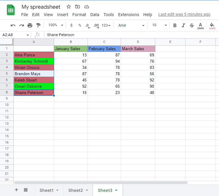
What if you want to evaluate multiple cells and then highlight cells based on the result? For example, suppose there is a data set that looks like this:

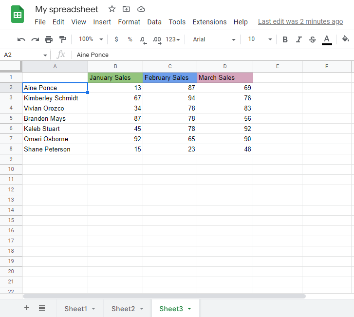
For example, if you are a business owner and want to highlight the salesperson who has yet to reach the monthly quota for the last three months, you can do so by highlighting the names of the salesperson who has sold more than 50 products in three months.

Here are the methods you need to take:

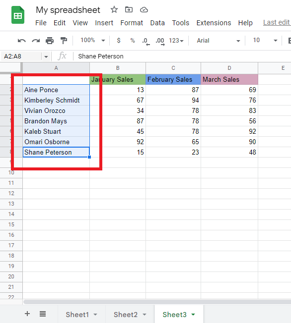
Select the cells "A2:A8."
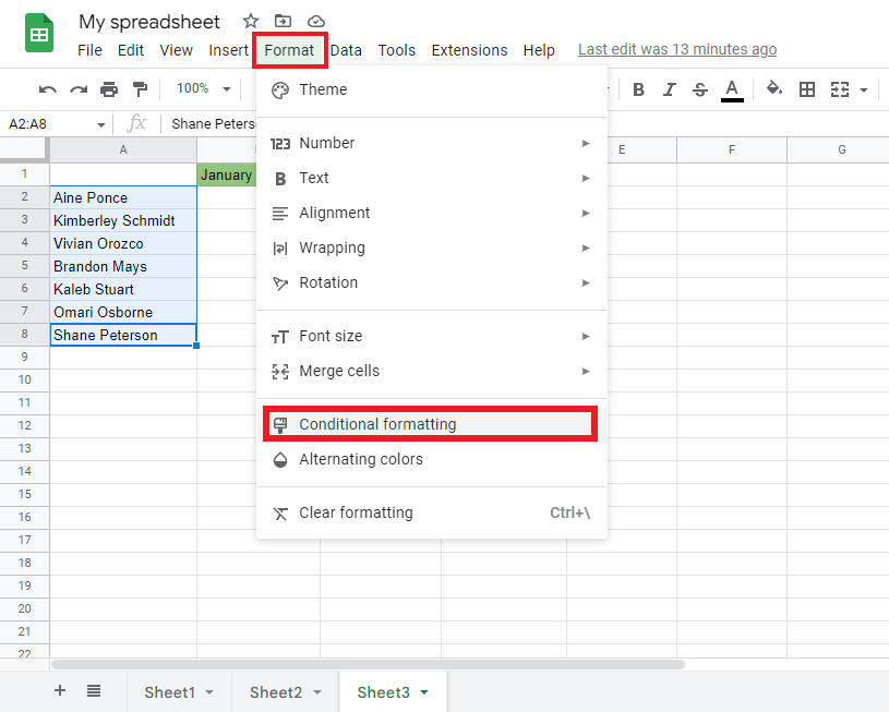
Find and click the "Format Tab" and click Conditional Formatting.
At the Conditional Formatting rules pane, Select Color and locate the "Format Cells if" drop-down.
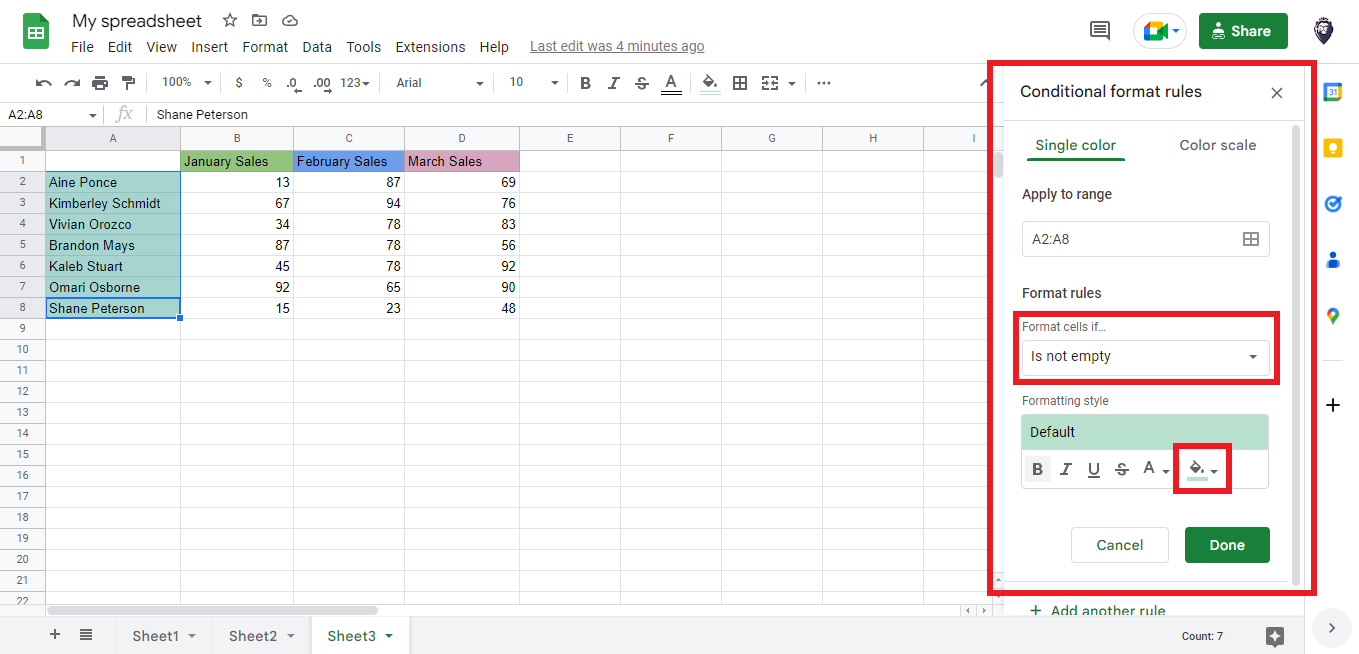
Select "Custom Formula."
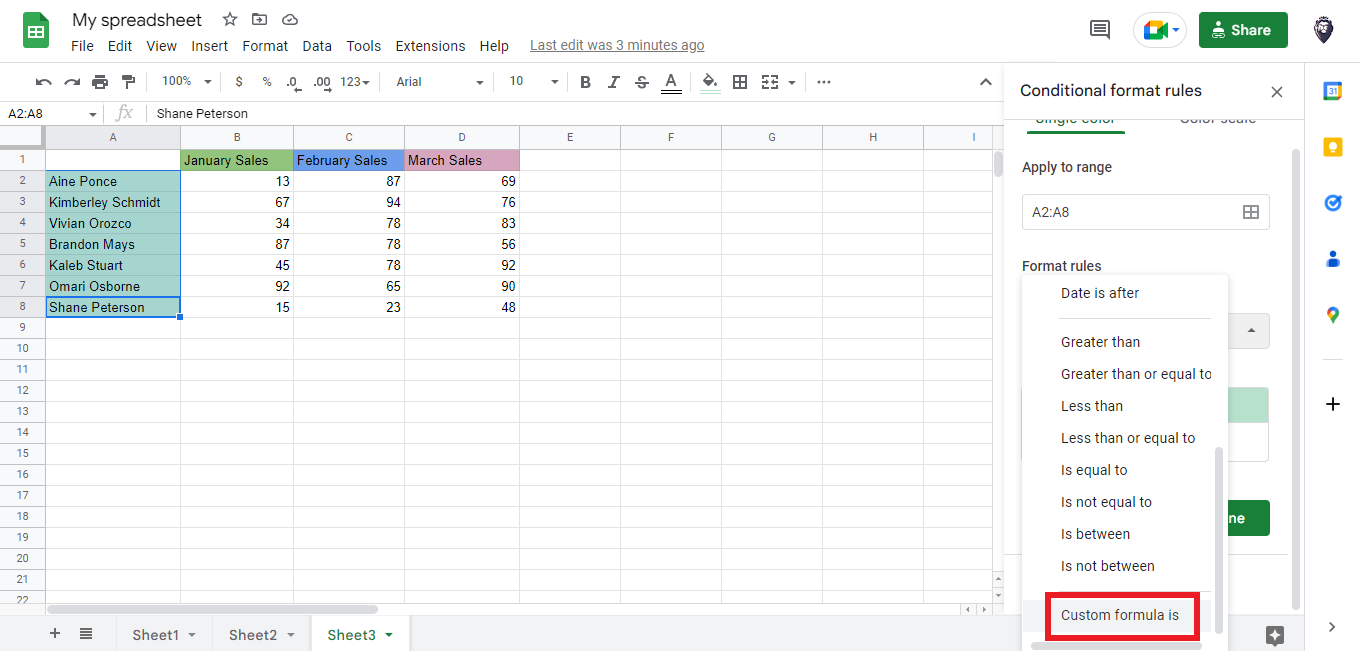
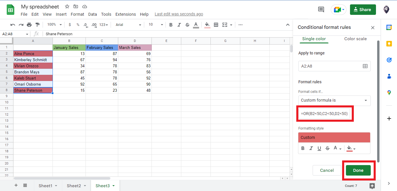
At the "Formula/Value" bar, enter the formula: =OR(B2<50, C2<50, D2<50), and click on Done.
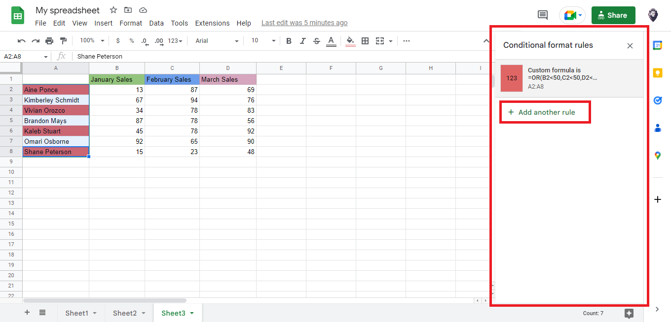
Go to the "Conditional Formatting Pane" and click the "Add new rule" button.
In the "Format Cells if" drop-down, select "Custom Formula is." In the Formula/Value bar, enter the formula: =AND(B2>60, C2>60, D2>60), and click "Done."
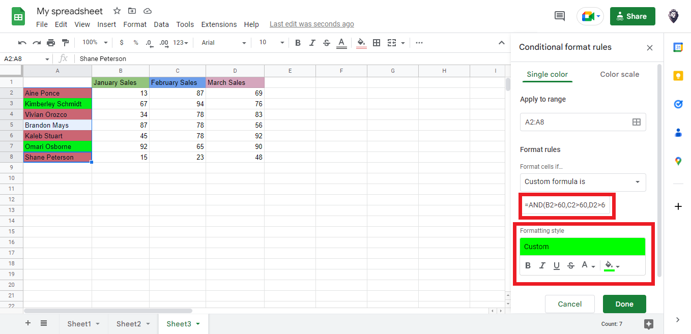
Google Sheets will show the names in a different color, like this:

How to use Google Sheets Conditional Formatting if Another Cell Contains Text.

You can add conditional formatting in Google Sheets based on another cell containing text. You must enter the text string into quotation marks in the custom formula.

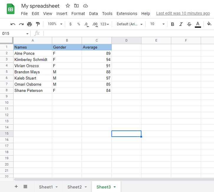
Perhaps you work in a primary school. Finding top-performing male students for an all-boys private school scholarship program would be best. To do this, you can use conditional formatting to highlight all male students on your list.

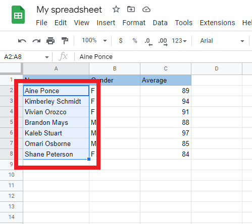
Select cells A2:A8.

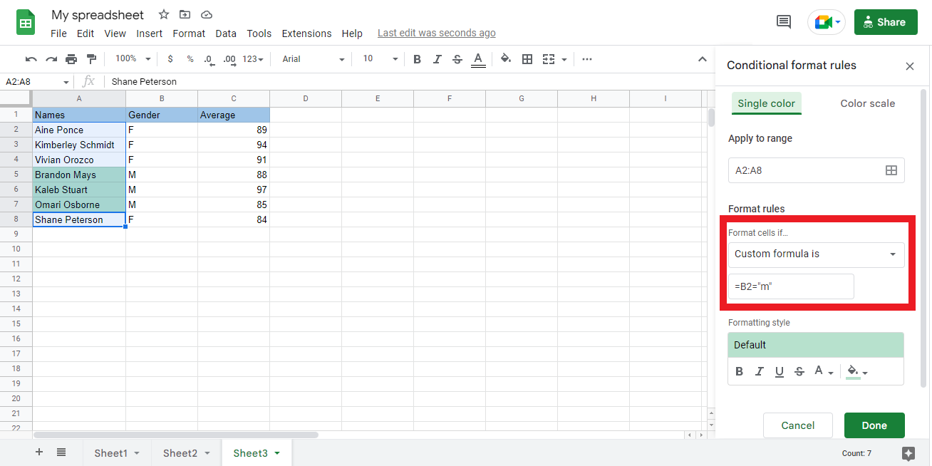
Locate the "Format" tab, and go to the "Conditional formatting" option.

Click the "Conditional drop-down box," change it to "Custom formula is," Enter B2=" M," and click "Done."

Final Thoughts on Google Sheets Conditional Formatting Based on Another Cell

Now you have three different methods of conditional formatting based on another cell. It improves your skill with Google Sheets and makes formatting cells much more accessible.

You can visit our homepage for more easy-to-follow how-to and step-by-step guides. Check the related articles section links for further details about Excel/Google Sheets Templates!

Frequently Asked Questions on Google Sheets Conditional Formatting Based on Another Cell:

How do I conditional format a cell based on another cell in Google Sheets?

To conditionally format a cell based on another cell in Google Sheets, select the "Format" menu and choose "Conditional Formatting."

What are the different options for conditional formatting in Google Sheets?

You can use different options, such as text, cell, or date conditions, to make numbers stand out if they are above or below a certain amount; change the Color of the background of a cell if it has a specific word, or add designs to cells based on dates.

How do I use multiple conditions for conditional formatting in Google Sheets?

Choose the cell or range of cells you want to format, then click 'Format' and choose 'Conditional Formatting.' From here, you can specify the conditions that trigger the formats by clicking on any of the existing rules or adding a new one, and after you do this, all that is left to do is define your custom formats!

What are Google Sheets: Uncover the Essentials You Need to Know

How to Use Google Sheets: Everything You Need to Know

Google Sheets Filter Function: How and When to Use One

Want to Make Excel Work for You? Try out 5 Amazing Excel Templates & 5 Unique Lessons

We hate SPAM. We will never sell your information, for any reason.