How to Remove Duplicates in Google Sheets Without Using Apps Script

Whether you're a small business owner or a spreadsheet god that uses Excel for data analysis, there's no beating around the bush that Google Sheets has now been a staple for all sorts of people and organizations when it comes to fulfilling their spreadsheet needs. Who can blame them? Auto-saves, collaboration, and the free price tag do come in handy. That being said, many differences exist in how different functions and tools operate between both applications. With the integration of Google Sheets with another app, such as Google Forms, we see more and more raw data being processed with Google Sheets. For example, if you use a Google Sheet to track attendance, you will have duplicate values, whether text or numbers. In this article, we'll talk about a few neat tricks we can use in Google Sheets to highlight duplicates, identify duplicates, and remove duplicates in Google Sheets.

How to Highlight Duplicate Cells in or Within a Single Column Range

Duplicates in Google Sheets: Not as Straightforward as You Think Suppose we maintain a list with names in Google Sheets, and we want to see which duplicate entries there are so we can take note of returning customers. 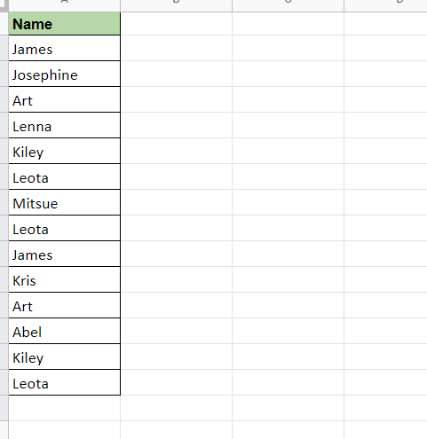Manually checking for duplicate entries in this list is not only time-consuming but also very prone to errors. As we mentioned earlier, there are many things that Google Sheets does differently from Microsoft Excel. One of these things is readily highlighting duplicates using conditional formatting. In Excel, you can underline duplicates in as easy as three clicks. Highlighting duplicates in Google Sheets requires a couple more steps.

Step-by-Step: How to Highlight Duplicate Entries In a Single Column In Google Sheets

Step 1: Select the data range to highlight duplicate entries or note their column letter. 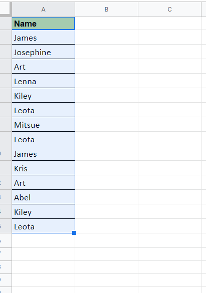Note: When creating your selection, be mindful of the header row, as its formatting could change depending on if there's a duplicate somewhere in the range. Step 2: Open up the conditional formatting module. In the Menu Bar, select Format, and in the dropdown, select Conditional Formatting to open up the conditional formatting module. 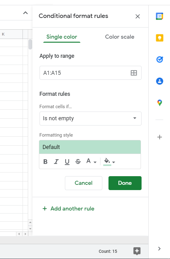Step 3: Create a custom formula. Unlike Excel, Google Sheets doesn't have a preset condition to highlight duplicates, so we must create our own. Select "Custom formula is" in the Format Rules dropdown. 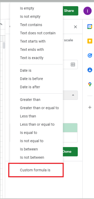Enter this formula: =COUNTIF(A:A,A1)>1 This formula allows you to highlight duplicate cells in a single column. 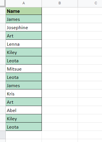Note that any new entries entered at the bottom will not be included unless you adjust the "Apply to range" field in the Conditional Format Rules Module.

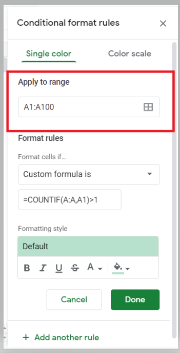
How it Works:

This custom formula creates a true/false check. We can see this custom formula in action if we place it beside the column with duplicate records we worked on. 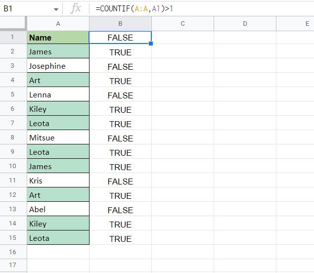We see that it returns a True or a False value. Here, we used the COUNTIF statement to get the number of instances a name appears in the column. When we add the ">1," we tell Google Sheets to return True if the number of cases is more than one and False if not. When we plug this in the conditional formatting module, the custom formula adds Color to the cells involved if there is more than one instance of it or duplicates.

Step-by-Step: Highlighting Duplicate Data Across Multiple Columns

If you want to highlight duplicate data in a data range that spans multiple columns, you can use the steps above with just some variations to the custom formula. Suppose we have two columns now that we want to check for duplicate data. 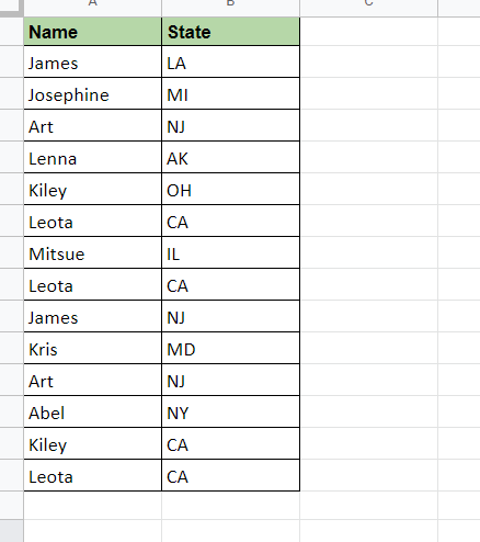Step 1: Select the columns we want to apply the conditional formatting. 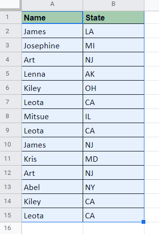Step 2: Open the Conditional Format Rule Module. As we did earlier, in the Menu Bar, select Format, and in the dropdown, select Conditional Formatting to open up the conditional formatting module. Step 3: Create your custom formula. In the Format Rules portion, select again "Custom formula is." 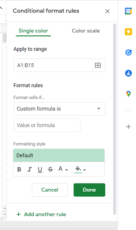Enter this formula =COUNTIF(A:B,A1)>1 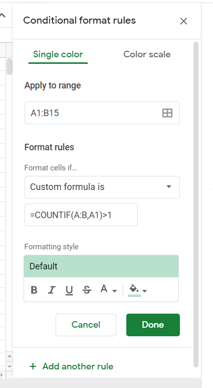Your selected columns now have the duplicate values highlighted! 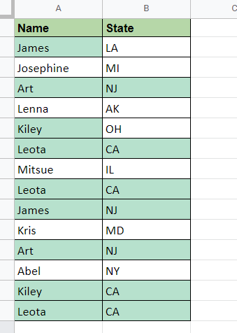Without having the preset, it just takes a bit longer to highlight duplicates in Google Sheets, but with a little Excel know-how, you will also master Google Sheets like the back of your hand. In the next section, let's discuss how to delete duplicates or remove duplicate rows.

How to Remove Duplicates in Google Sheets

Using the Filter Tool

Knowing how to delete duplicates would be one of the more critical skills if you're trying to maintain a database. If you're coming from the previous section and know how to highlight duplicates, you can use the Filter tool in Google Sheets to remove duplicates manually. This method deletes copies based on cell formatting, so it's a given that you need to format cells as a prerequisite. Step 1: Select a cell inside the data range and create a filter. Click on any cell within your data range, and in the Menu Bar, open the Data Menu dropdown and select "Create Filter." 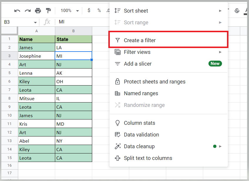You can tell if you've correctly created the Filter by seeing the filter options icon on the header row. 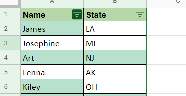Step 2: Filter out the unique rows. Open the filter options icon of the column where you want to see duplicate rows. Select Filter by Color> Fill Color and select the Color you set for the highlighted duplicates. 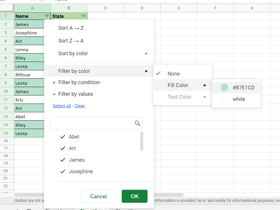You should see something like this. 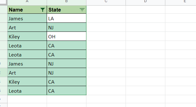Step 3: Manually remove duplicate cells. Start reviewing and manually deleting duplicate rows starting from the bottom. You can select an entire column using the keyboard shortcut Shift + Space Bar. 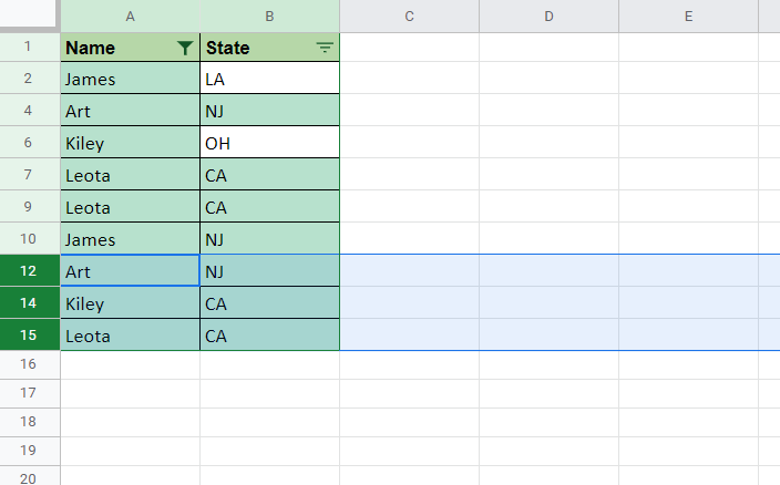You can tell when you have the whole duplicate rows selected if the row number on the left is highlighted. To delete duplicate rows, go to the Menu Bar > Edit > Delete > Delete Selected Rows 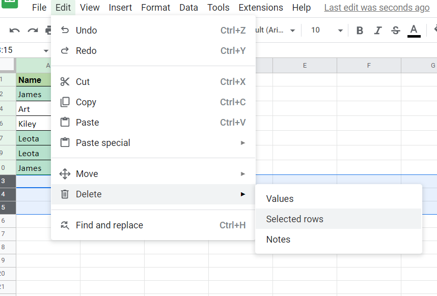As you remove duplicate rows, the original values lose their formatting, indicating that only one unique value remains for that cell in the data set. 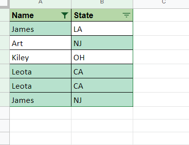This method can be used to analyze an entire table, but it works best with fewer rows as this takes a lot of time. However, this method allows you to check before you delete entire rows individually. It's also important to note that this could take Google Sheets more time to process, depending on how many duplicates are present.

Using the Built-in Remove Duplicates Tool

With the manual method of removing duplicates in Google Sheets, we can now get down to business to remove duplicate entries. This is the fastest method of deleting copies in Google Sheets. Step 1: Select your table. 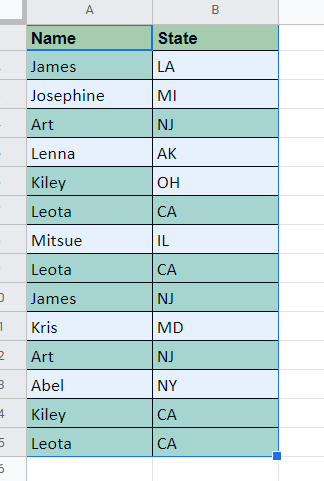Step 2: Open up the Remove Duplicates tool. In the Menu bar, open the Data Menu and select Data Cleanup, then Remove Duplicates. 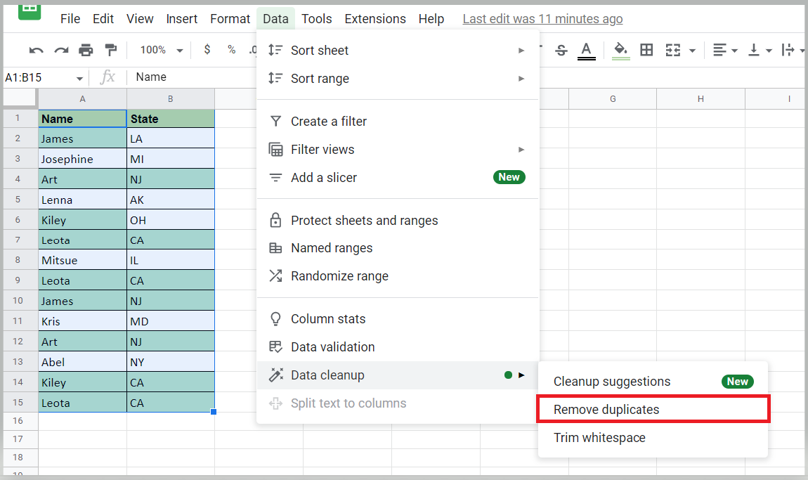Step 3: Set your parameters and remove duplicates. The Remove Duplicates Dialog Box appears, and here we can select the column or columns to seek out the duplicates from. 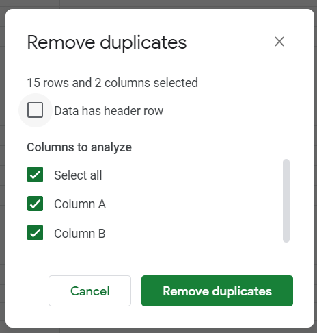We can tick the check box on top to tell the tool whether or not our selected data range contains headers. Once we tick that check box, we can see the column names appear in the Columns to analyze portion. 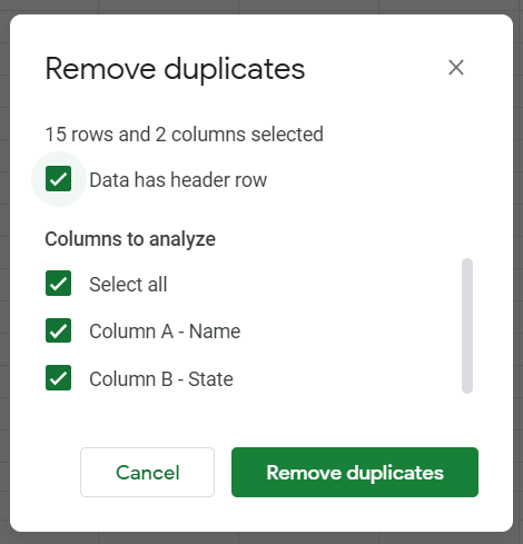Suppose you only want to remove duplicates based on the names. We can untick "Column B - State" and press Remove Duplicates. 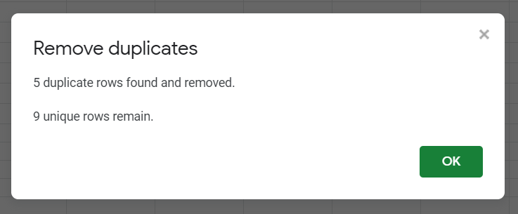A message shows you how many duplicate rows were found and how many remain. 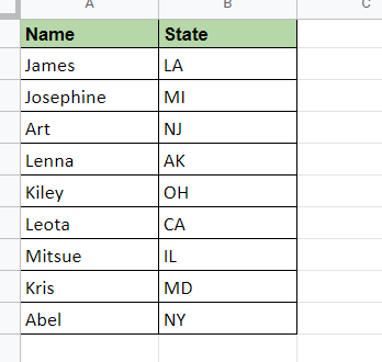As we can see above, only the deduplicated data in the list remain. The conditional formatting that we set a while ago is now gone indicating that all we see are unique rows. Do note that the tool operates by deleting rows from the bottom of the table going up, similar to what we did a while ago during the manual removal.

Removing Duplicates Using the UNIQUE Function

Another less-invasive way of removing duplicate rows in Google Sheets is using the UNIQUE function. The UNIQUE function is an array function that returns only one instance of each unique value in a given data range. This array function is dynamic and fully automatic, making it great for use in dashboards and automated spreadsheets. Like our previous examples, let's try getting the unique names in this list. 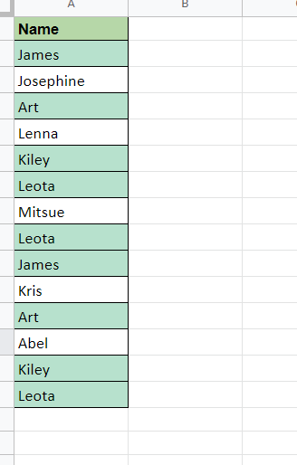In a separate column, let's type in this formula: =UNIQUE(A2:A15) 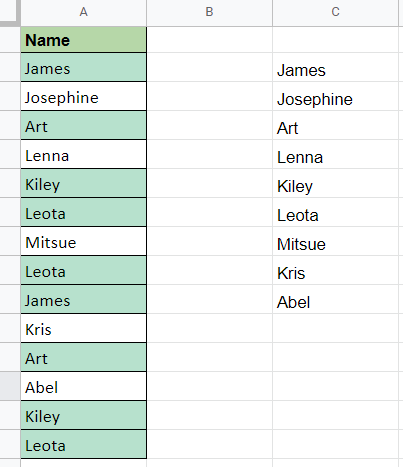As we can see, it only returned the unique names in the list, effectively removing the same data. This method allows you to work indirectly off a data set which allows you to preserve its integrity. Suppose we were to use the Remove Duplicates tool on our primary data set. In that case, it'd be tough to ensure the integrity of the data when we delete a duplicate row, whereas using this function allows you to remove duplicates while leaving the data alone. When using dynamic array formulas, it's essential to ensure that the cells under the cell that has the procedure are clear if values or text are under the primary cell, a #REF! Error appears. 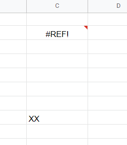This error is the equivalent of the #SPILL! Error in Microsoft Excel. In our other blog post, you can't find a guide on dealing with that.

The Wrap-Up

Whether you're team Microsoft Excel or Team Google Sheets, both applications have quirks and methods of getting things done. This article lets you extract unique records in your existing sheet, compare columns for duplicate entries, and know how to remove duplicates in Google Sheets.