
How to Add a Drop-Down List in Excel
Feb 06, 2026
Summary: How to Make a Drop Down List in Excel
Learning how to create a drop down in Excel is the best way to speed up data entry and prevent spelling errors. This guide provides a complete walkthrough on adding these validation lists to your spreadsheets. You will learn the four main methods: using comma-separated values for simple yes/no options, referencing cell ranges for standard lists, utilizing Excel Tables for dynamic lists that update automatically, and leveraging spill arrays for advanced filtering.
Additionally, we cover how to customize your drop down box in Excel with input messages to guide users and error alerts to stop invalid data. Whether you need a simple selection or a complex dependent drop down list, this tutorial has you covered.
Table of Contents

Creating a drop down list in Excel (also known as a picklist) makes data entry faster and improves usability.
A drop down menu in Excel allows users to select a value from a predefined list instead of manually typing it. It helps streamline data entry, reduce errors, and ensure consistency in spreadsheets. This is particularly useful for forms, reports, and data validation requiring standardized inputs.
This guide will walk you through everything you need to know, from how to insert a drop down list in Excel to advanced techniques like dynamic and dependent drop-down lists.
Get our free Excel formulas cheat sheet
Plus new tutorials and template drops. Enter your email and we'll send it over.
Creating Simple Drop-Down Lists
You don't need to be a tech expert to add a drop down in Excel. Excel's Data Validation feature makes the process super easy.
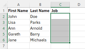
Our sample file contains the names of people. We want to write each individual's job and create a selection list in Excel so that the user selects the job instead of writing it manually. For BOMs specifically, our bill of materials excel template uses this dropdown pattern for SKU selection.
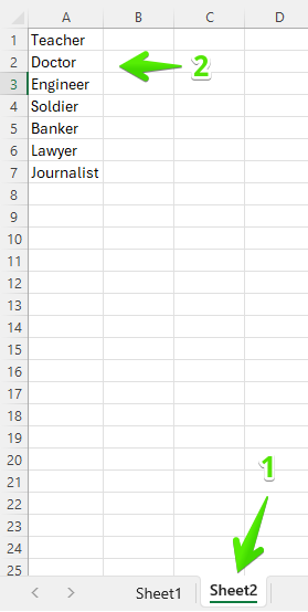
Step 1: Prepare the source list.
Before you create drop a down menu in Excel, you need to organize the source data that will populate the list. We recommend that you do this in a new sheet. For example, if you are doing the main work in Sheet1, you should enter your source list in Sheet2.
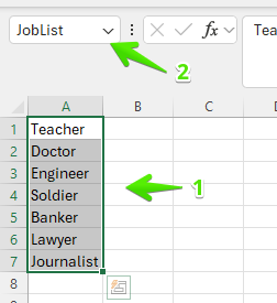
To make your work smarter and create list in Excel efficiently, select the entire list (e.g., A1:A7 in Sheet2). Click the Name Box (the small box to the left of the formula bar). Type a name (e.g., JobList) and press Enter. This makes it easier to reference the list later.
Step 2: Select the target cells.
Return to the main sheet and select the cell(s) where you want the Excel dropdown to appear. You can select single or multiple cells, depending on your needs.
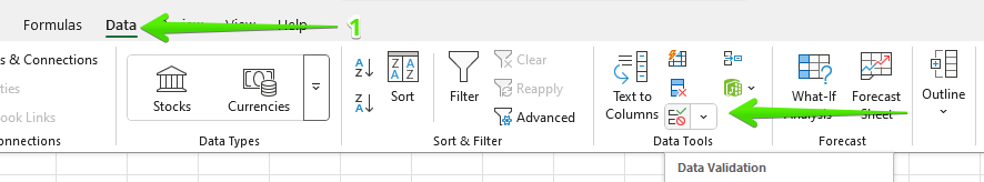
Step 3: Open the Data Validation menu.
Click on the Data tab in the ribbon. Select Data Validation from the Data Tools group. This will open the Data Validation dialog box where you configure your Excel pick from drop down list settings.
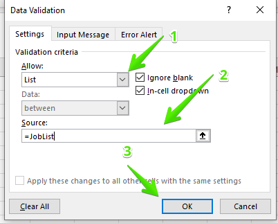
Step 4: Set up the validation criteria.
In the Data Validation window, go to the Settings tab. Under Allow, choose List from the drop-down menu. Then, click inside the Source box and type the formula =JobList (if you named your range earlier). If you didn’t name the range, use this format instead: =Sheet2!A1:A7. Finally, ensure Ignore blank and In-cell dropdown are checked.
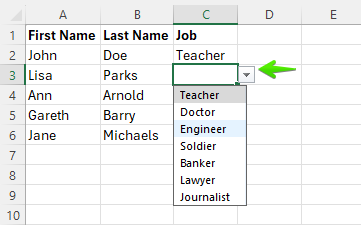
Step 5: Test the drop-down list.
Your Excel dropdown list in cell should now be active. Click on a cell to see a small arrow appear, then select it to excel choose from list.
Comparison of Drop-Down Methods
There are several ways to do a drop down list in Excel depending on your data needs. Here is a quick comparison to help you choose the best method.
| Method | Best For | Dynamic? | Complexity |
|---|---|---|---|
| Manual Entry (Comma-separated) | Short, static lists (e.g., Yes/No, High/Low) | No | Low |
| Cell Range Reference | Standard lists that change occasionally | No (unless range is updated) | Low |
| Excel Table | Lists that grow/shrink often (Recommended) | Yes (Auto-updating) | Medium |
| Spilled Array (#) | Lists generated by formulas like UNIQUE or SORT | Yes (Fully dynamic) | High |
Pro Tip: Create an Auto-Updating (Dynamic) Drop-Down List
The standard method above works great, but it has one flaw: if you add a new item to the bottom of your source list later, the drop down box in Excel won't automatically include it. You would have to update the range manually.
To fix this, turn your source list into an Excel Table:
- Select your source list (e.g., the job titles in Sheet2).
- Press Ctrl + T (or go to Insert > Table) and click OK.
- Click inside the Data Validation Source box again.
- Highlight the list items in the table (not the header). Excel will usually insert a specialized reference like
=Table1[JobTitles].- Note: If Excel refuses the Table name reference directly in Data Validation (older versions), use the INDIRECT function:
=INDIRECT("Table1[JobTitles]").
- Note: If Excel refuses the Table name reference directly in Data Validation (older versions), use the INDIRECT function:
Now, whenever you type a new job title at the bottom of that table, your Excel drop down from list will instantly update to include it! For tracking stock, this technique pairs well with our inventory management template.
Using Spilled Arrays (Excel 365)
If you are using modern Excel functions like =UNIQUE() or =SORT() to generate your list, you can reference the entire "spilled" list using a single hash symbol (#).
- Suppose your
UNIQUEformula is in cell D1. The results "spill" down into D2, D3, etc. - In the Data Validation Source box, simply type:
=$D$1# - This tells Excel to "look at D1 and everything that spills from it." If the formula results expand, your excel dropdown expands with them.
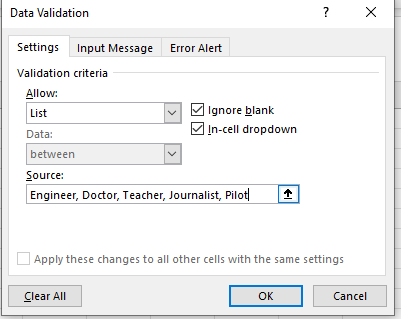
Alternative method: Enter list items directly.
Instead of referencing a range, you can type your items directly into the Source box to create options in Excel manually. This is useful for short lists that won’t change often. Ensure you separate the items with commas. For example:

Adding Input Messages and Error Messages Using Data Validation
Another cool feature when creating dropdowns in Excel is that you can customize an input message to guide users and an error message to prevent invalid data entry.
How to add an input message.
This instructs Excel to show a small pop-up displaying a message whenever a user selects a cell. Follow the steps below:
- Select the cell(s) where you have applied Data Validation.
- Go to the Data tab in the Excel ribbon and click Data Validation.
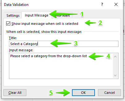
- In the Data Validation window, go to the Input Message tab.
- Check the "Show input message when cell is selected" box.
- Enter a title (optional, e.g., "Select a Category").
- Enter the message in the text box (e.g., "Please select a category from the drop-down list.").
- Click OK.
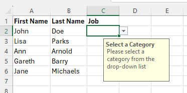
Result:
How to add an error message.
When you add picklist to Excel, creating an error message ensures data integrity. Here's how:
- Select the cell(s) with the drop-down list.
- Go to the Data tab and click Data Validation.
- Open the Error Alert tab.
- Check the "Show error alert after invalid data is entered" box.
- Choose a Style:
- Stop (default) – Prevents users from entering invalid data.
- Warning – Displays a warning but allows invalid data.
- Information – Informs users but still accepts invalid data.
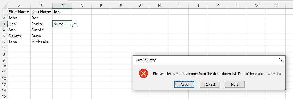
- Enter a title (e.g., "Invalid Entry").
- Enter the message (e.g., "Please select a valid category from the drop-down list. Do not type your own value.").
- Click OK.

Result:
Tip: How to Allow Users to Type Custom Text
Sometimes you want to suggest a list of options but still allow the user to type their own value (like "Other").
- Go to the Error Alert tab in Data Validation.
- Uncheck the box that says "Show error alert after invalid data is entered."
- Click OK. Now users can pick from the list OR type a custom entry without receiving an error message.
How to Color-Code Your Drop-Down Selections
A common request is to have the cell change color based on the item selected (e.g., Green for "Approved," Red for "Rejected"). You can do this with Conditional Formatting. For task tracking specifically, our task tracker excel template uses this exact dropdown pattern.
- Select the cell(s) containing your drop-down list.
- Go to Home > Conditional Formatting > Highlight Cell Rules > Equal To...
- Type the list item (e.g., "Approved") and choose a color (e.g., Green Fill).
- Repeat this process for other items in your list. Now, your drop-down isn't just functional; it's visual!
How To Create a Dependent Drop Down List
A dependent drop down list is where options change based on a selection from another list. This is useful for hierarchical data like Category → Subcategory (e.g., selecting "Fruit" shows only fruits). This same Product → Line pattern is how a production planner excel filters daily output by line or shift.
Step 1: Prepare your data.
Structure your data properly before setting up the dependent drop-down list.
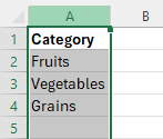
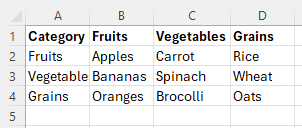
1. Create the main category list (e.g., in Sheet2, Column A):
2. Create subcategory lists for each category in separate columns:
Step 2: Name the ranges.
Named ranges make it easier to reference the subcategories.
- Select the main category list (e.g., A2:A4).
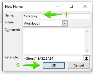
- Go to the "Formulas" tab and select "Define Name".
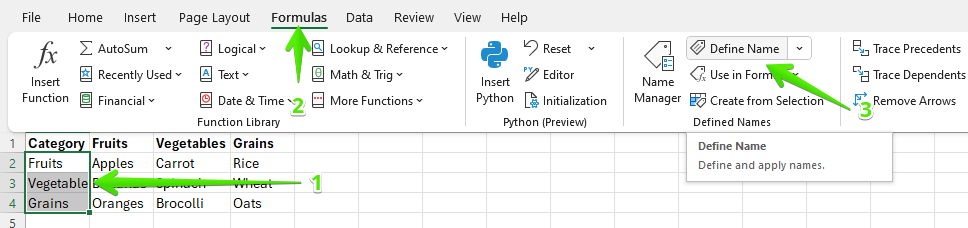
- Enter a name (e.g., Category) and click OK.
Now, define named ranges for each subcategory:
- Select the subcategory items under "Fruits" (B2:B4).
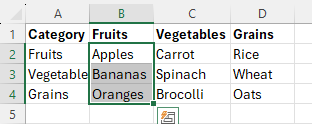
- Go to "Formulas" → "Define Name" and enter Fruits as the name (it must match the category name exactly).
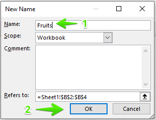
- Repeat this for Vegetables (C2:C4) and Grains (D2:D4), naming them as Vegetables and Grains, respectively.
Step 3: Create the first drop-down list (Main category).
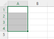
- Go to the sheet where you want the drop-down lists.
- Select the cells to which you want to apply the first dropdowns.
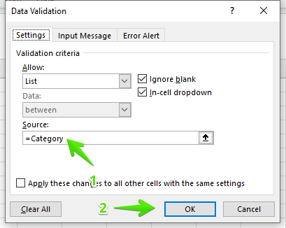
- Click Data → Data Validation.
- Under Allow, select List.
- In the Source field, enter:
=Category - Click OK.
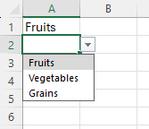
Result:
Step 4: Create the dependent drop-down list.
- Select the cells for the dependent drop-downs.
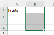
- Click Data → Data Validation.
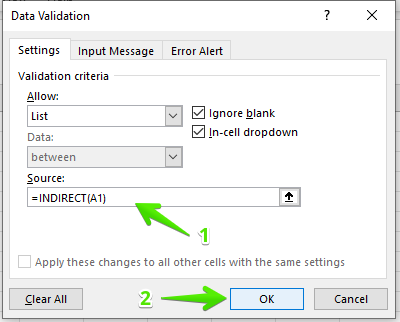
- Under Allow, select List.
- In the Source field, enter:
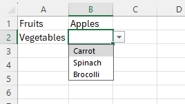
=INDIRECT(A1) - Select OK.
Result:
How to Edit or Change an Existing Drop-Down List
If you need to change drop down list in Excel, add items, or remove them, you don't need to start over. Here is how to update a drop down list in Excel:
- Select the cell(s) containing the drop-down list.
- Go to Data > Data Validation.
- In the Source box, simply edit your range (e.g., change
=$A$1:$A$5to=$A$1:$A$10) or add new items to your comma-separated list. - Click OK.
Note: If you checked "Apply these changes to all other cells with the same settings," Excel will update every drop-down list that uses this source at once!
Quick Tip: The "Pick From Drop-down List" Feature
Did you know Excel has a hidden drop-down tool that requires zero setup? If you have a column of data (e.g., a list of cities in cells A1:A10) and you want to type one of those cities into cell A11, you don't need Data Validation.
- Right-click the empty cell directly below your list.
- Select Pick From Drop-down List... (or press Alt + Down Arrow).
- Excel will automatically show a list of all unique values from the cells directly above.
Final Thoughts
Using excel set drop down list features standardizes data entry, reduces errors, and improves user experience. Excel offers multiple ways to customize drop-downs to your needs, and we have covered each of them. Start with a basic list, and as you grow comfortable, explore dynamic and dependent lists for more automation and efficiency.
For more easy-to-follow Excel guides and the latest Excel Templates, visit Simple Sheets and the related articles section of this blog post. Vendor lookups in a purchase order template work exactly this way — try our purchase order template with vendor dropdowns to skip building one.
Subscribe to Simple Sheets on YouTube for the most straightforward Excel video tutorials!
Frequently Asked Questions (FAQ)
1. How do I remove a drop-down list in Excel?
To remove a drop-down list, select the cell(s), go to Data > Data Validation, and click Clear All in the dialog box. This removes the drop-down but keeps existing values in the cells.
2. Can I create a drop-down list with multiple selections?
Excel does not support multi-select drop-downs by default, but you can use VBA (Visual Basic for Applications) to allow multiple selections in a single cell. Alternatively, consider using checkboxes for better usability.
3. Why is my drop-down list not showing all options?
This can happen if the source range is incorrect or not formatted as a dynamic list. Check the Data Validation settings and ensure your range includes all intended items. Using an Excel Table as your source is the best way to prevent this.
4. Can I enable searching in a drop-down list?
In newer versions of Excel (Excel 365), drop-down lists are searchable by default. As you type in the cell, the list filters to match your text. For older versions, you would need complex formulas or a "Combo Box" form control to achieve this.
5. Can I copy my drop-down list to other cells?
Yes. You can simply copy the cell with the drop-down (Ctrl + C) and paste it (Ctrl + V) into other cells. If you want to copy only the drop-down without changing the cell formatting, use Paste Special > Validation.
6. Can I use a drop-down list to control a chart?
Yes! This is a powerful feature for dashboards. By linking your drop-down list to a cell, and then driving your chart data from that linked cell (using formulas like XLOOKUP or INDEX/MATCH), you can create interactive charts that update instantly whenever a user selects a different option from the list.
7. How do I make a dynamic list without using Excel Tables?
If you cannot use Excel Tables (the preferred method), you can use the OFFSET function. You would define a Named Range using a formula like =OFFSET(Sheet1!$A$1,0,0,COUNTA(Sheet1!$A:$A),1). This counts the non-blank cells in the column and adjusts the range height automatically, though it is more complex to set up than the Table method.
Related Articles & Resources
Get our free Excel formulas cheat sheet
Plus new tutorials and template drops. Enter your email and we'll send it over.
Want to Make Excel Work for You? Try out 5 Amazing Excel Templates & 5 Unique Lessons
We hate SPAM. We will never sell your information, for any reason.

