How to Calculate Percentage Change in Excel: Formula, Negatives and Errors
Feb 09, 2026
Short answer: what is the percent change formula in Excel?
The percent change formula in Excel is =(new-old)/old. Enter it in a blank cell, then click Percent Style on the Home tab to display the result as a percentage. Do not multiply by 100 as well, or you will get 5000% instead of 50%. If the old value can be zero, wrap it in IFERROR.
Last updated: August 18, 2026
Get our free Excel formulas cheat sheet
Plus new tutorials and template drops. Enter your email and we'll send it over.
Table of Contents
- What is the percent change formula in Excel?
- Percentage formula reference table
- How to calculate percent change step by step
- Percent change vs percent difference vs percentage increase
- Should you multiply by 100 or format as a percentage?
- How do you handle negative numbers?
- How do you stop the #DIV/0! error?
- Month over month and year over year down a column
- Why you cannot average percentages, use CAGR
- How to increase or reduce a number by a percentage
- Percentage points vs percentage change
- Red and green arrows with conditional formatting
- Common errors to avoid
- Frequently asked questions
What is the percent change formula in Excel?
Percent change measures how much a value has moved relative to where it started. The formula is always the same whether the number went up or down:
Percent change = (new value - original value) / original value
In Excel, with the old value in A2 and the new value in B2:
=(B2-A2)/A2
That returns a decimal such as 0.5. Applying the Percent Style format turns it into 50%. There is no dedicated PERCENTCHANGE function in Excel, so this arithmetic is the whole trick.
Rule: the denominator is always the starting value, never the ending value and never the average. Swap them and you get a different number that answers a different question.
Percentage formula reference table
Most percentage questions in Excel are one of these twelve formulas. Bookmark this table and you will rarely need to think about it again.
| What you want | Formula | Format the cell as |
|---|---|---|
| Percent change between two numbers | =(B2-A2)/A2 |
Percentage |
| Percent change that will not error | =IFERROR((B2-A2)/A2,"") |
Percentage |
| Percent change with negative starting values | =(B2-A2)/ABS(A2) |
Percentage |
| Percent difference between two numbers | =ABS(B2-A2)/AVERAGE(A2,B2) |
Percentage |
| Percent of a total | =A2/SUM($A$2:$A$100) |
Percentage |
| Increase a number by a percentage in a cell | =A2*(1+B2) |
Number or currency |
| Add a fixed 20% | =A2*1.2 |
Number or currency |
| Subtract a fixed 15% | =A2*(1-15%) |
Number or currency |
| Month over month change | =(B3-B2)/B2 filled down |
Percentage |
| Year over year change on monthly data | =(B14-B2)/B2 filled down |
Percentage |
| Average annual growth rate (CAGR) | =(B10/B2)^(1/8)-1 |
Percentage |
| Variance against budget | =(Actual-Budget)/ABS(Budget) |
Percentage |
How to calculate percent change in Excel, step by step
Here is the calculation on real numbers. January sales are in A2 and February sales are in B2.
1. Enter your two values. Put 100 in A2 and 150 in B2.
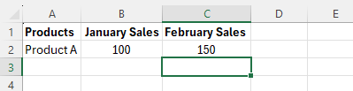
2. Click the cell where the answer goes. In this example, C2.
3. Type the formula. Enter =(B2-A2)/A2 and press Enter. C2 shows 0.5.
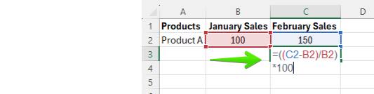
4. Format it as a percentage. With C2 selected, press Ctrl + Shift + %, or click Percent Style in the Number group on the Home tab. C2 now reads 50%.
5. Fill it down. Double-click the small square at the bottom right of C2 and Excel copies the formula down alongside your data.
Microsoft covers the underlying number formatting behaviour in Calculate percentages.
Percent change vs percent difference vs percentage increase
These three phrases get used interchangeably and they are not the same calculation. Picking the wrong one is the most common reason two people analysing the same data report different numbers.
| Measure | Formula | Denominator | 40 to 50 gives | Use it when |
|---|---|---|---|---|
| Percent change | =(B2-A2)/A2 |
The starting value | 25% | One thing measured at two points in time |
| Percentage increase | =(B2-A2)/A2 |
The starting value | 25% | Same as percent change, just named for the direction of travel |
| Percentage decrease | =(B2-A2)/A2 |
The starting value | 50 to 40 gives -20% | Same formula, the sign tells you the direction |
| Percent difference | =ABS(B2-A2)/AVERAGE(A2,B2) |
The average of both values | 22.2% | Two independent things compared to each other, with no before and after |
Notice that percentage increase and percentage decrease are not separate formulas. They are the same subtraction, and the minus sign does the work. Percent difference is the genuine outlier: it is symmetric, so comparing A to B gives the same answer as comparing B to A, which percent change never does.
Rule: if one of the two numbers came first in time, you want percent change. If neither did, for example two suppliers' prices or two machines' output, you want percent difference.
Should you multiply by 100 or format as a percentage?
Format as a percentage. Multiplying by 100 is the single most common source of wrong-looking percentage results in Excel.
=(B2-A2)/A2returns 0.5. Apply Percent Style and the cell shows 50%, and the stored value is still 0.5, so downstream maths keeps working.=((B2-A2)/A2)*100returns 50. If the cell is already formatted as a percentage, or someone formats it later, it will display as 5000%.
The second problem is chaining. If you multiply by 100 and then feed that cell into another calculation that expects a rate, everything downstream is out by a factor of 100. Keep percentages stored as decimals and let the number format do the presentation.
Shortcut: Ctrl + Shift + % applies Percent Style instantly. To show one decimal place, use a custom format of 0.0%.
Rule: store the rate, format the display. If you can see both a percent sign and a multiplication by 100 in the same column, one of them is wrong.
How do you handle negative numbers in a percent change formula?
This is where the standard formula quietly breaks, and it matters because profit, cash flow and budget variance columns are full of negative numbers.
Take a loss that shrank from -50 to -25. That is a genuine improvement. The standard formula gives:
=(-25 - -50)/-50 which is 25/-50, or -50%
Excel says the number went down 50% when the business actually got better. The negative denominator flipped the sign. The fix is to divide by the absolute value of the starting number:
=(B2-A2)/ABS(A2)
That now returns +50%, which correctly says the loss halved. Use this version in any column that can contain negatives.
When the sign flips from negative to positive
If the old value is negative and the new value is positive, for example a loss of -20 turning into a profit of 30, percent change is mathematically meaningless. There is no percentage that describes crossing zero. Reporting "250% growth" there is wrong, and finance reviewers will catch it.
Flag those rows instead of computing them:
=IF(A2=0,"n/a",IF(SIGN(A2)<>SIGN(B2),"n/m",(B2-A2)/ABS(A2)))
"n/m" is the standard finance abbreviation for not meaningful, and it is what a proper variance report shows.
Rule: use ABS in the denominator whenever negatives are possible, and report a sign change as not meaningful rather than as a percentage.
How do you stop the #DIV/0! error?
If the starting value is zero or the cell is blank, =(B2-A2)/A2 divides by zero and Excel returns #DIV/0!. A single one of these poisons any SUM or AVERAGE further down the sheet, and it looks broken in a report.
Three ways to handle it, from simplest to most correct:
- Blank it out.
=IFERROR((B2-A2)/A2,"")catches every error type, not just division by zero, and leaves a clean empty cell. - Label it.
=IFERROR((B2-A2)/A2,"n/a")makes it obvious that no calculation was possible, rather than looking like a data gap. - Test the cause explicitly.
=IF(A2=0,"n/a",(B2-A2)/A2)only handles zero, so genuine errors elsewhere in the formula still surface instead of being swallowed.
Option three is the safest habit in financial models. IFERROR is a blanket, and a blanket can hide a real mistake such as a broken reference.
Rule: IFERROR hides every error, not only the one you were thinking of. In a model that matters, test for the zero directly with IF.
Related: The Excel IFERROR Function: what it is and when to use it
How do you calculate month over month and year over year change down a column?
Comparing one pair of cells is easy. The useful version is a whole column of changes next to a whole column of data. Say column A holds the month and column B holds the value, starting in row 2.
Month over month
In C3, enter =(B3-B2)/B2 and fill down. Leave C2 empty, because the first month has nothing before it to compare against. To make that self-documenting:
=IFERROR((B3-B2)/B2,"")
Year over year
With monthly data, this year's January sits twelve rows below last year's January. So in C14, enter =(B14-B2)/B2 and fill down. Every row now compares to the same month a year earlier, which strips out seasonality. Month over month says December beat November. Year over year tells you whether this December beat last December, which is the number that actually means something in a seasonal business.
If your data is not in tidy chronological rows, use a lookup instead of an offset so the comparison cannot silently break:
=IFERROR((B14-SUMIFS($B:$B,$A:$A,EDATE(A14,-12)))/SUMIFS($B:$B,$A:$A,EDATE(A14,-12)),"")
Rule: month over month measures momentum, year over year removes seasonality. Report both, because either one alone can tell a flattering story.
Why you cannot just average percentages, and what to use instead
Averaging a column of percent changes feels reasonable and is almost always wrong. Percentages compound, so they do not average arithmetically.
Take a value that rises 50% and then falls 50%. Start at 100, go to 150, then to 75. The arithmetic average of +50% and -50% is 0%, but you have lost a quarter of your money. The average is not just imprecise, it points the wrong way.
Use the compound annual growth rate instead. CAGR asks a different and better question: what single steady growth rate would have taken you from the start value to the end value over that many periods?
CAGR = (ending value / beginning value) ^ (1 / number of periods) - 1
With the start value in B2, the end value in B10 and eight periods between them:
=(B10/B2)^(1/8)-1
Format as a percentage. In the 100 to 150 to 75 example, CAGR over two periods is =(75/100)^(1/2)-1, or about -13.4% per period, which is the honest answer.
Two things to watch. Count periods, not data points: eleven annual figures are ten periods. And CAGR cannot cope with a negative or zero starting value, so fall back on absolute change there.
Rule: never average a column of percent changes. Up 50% then down 50% averages to 0% and actually loses 25%. Use CAGR.
How do you increase or reduce a number by a percentage?
This is the reverse operation: you know the rate and you want the new number.
- Increase:
=A2*(1+B2)where B2 holds the rate. To add a fixed 20%, use=A2*1.2. - Decrease:
=A2*(1-B2). To take 15% off, use=A2*(1-15%), which turns 100 into 85. - A whole column at once, without formulas: type the multiplier such as 1.2 into a spare cell, copy it, select your range, then Paste Special > Multiply. Every value is uplifted in place. Delete the spare cell afterwards.
Watch the direction. Adding 20% and then removing 20% does not return you to the original number, because the second percentage is taken from the larger figure. 100 becomes 120, then 96.
Percentage points vs percentage change
If an interest rate moves from 10% to 12%, that is a 2 percentage point increase, but a 20% percentage change. Both statements are true and they are not interchangeable. Mixing them up is one of the fastest ways to lose credibility in a report.
| Feature | Percentage Change | Percentage Points |
|---|---|---|
| Core Definition | Measures the rate of growth or decline relative to the starting value. | Measures the arithmetic difference between two percentage values. |
| Formula | =(New - Old) / Old |
=New_Percentage - Old_Percentage |
| Example Scenario | An interest rate increases from 10% to 12%. | An interest rate increases from 10% to 12%. |
| The Result | This is a 20% increase in the rate. | This is a 2 percentage point increase. |
| Best Used For | Financial growth, sales performance, and budget variances. | Reporting changes in interest rates, tax brackets, or survey results. |
Rule: if both of your numbers are already percentages, subtract them and say "percentage points". Only use percent change when the underlying values are counts, amounts or rates.
How do you show percent change with red and green arrows?
A column of percentages is hard to scan. Icon sets turn it into something a reader understands at a glance, and it takes about thirty seconds to set up.
- Select your percent change column.
- Go to Home > Conditional Formatting > Icon Sets and pick 3 Arrows (Colored).
- Excel splits the range into thirds by default, which is almost never what you want. Go back to Conditional Formatting > Manage Rules > Edit Rule.
- Set Type to Number for both thresholds, and enter 0 in each value box. Green up arrow now means above zero, red down arrow means below zero, yellow flat means exactly zero.
- Optionally tick Show Icon Only if the arrow is enough on its own, or leave it off to show the arrow next to the number.
If you would rather colour the number than add an icon, skip conditional formatting and use a custom number format instead. Press Ctrl + 1, choose Custom, and enter:
0.0%;[Red]-0.0%;"flat"
Positive values show in the default colour, negatives show in red, and an exact zero shows the word flat. Custom formats are faster than conditional formatting on very large sheets because Excel does not have to re-evaluate a rule for every cell.
Rule: set icon set thresholds to Number 0 and 0. Left on the default percentile split, the arrows describe the shape of your data rather than whether anything actually grew.
Related: Using Conditional Formatting in Excel and How to make negative numbers show up in red
Common errors to avoid when calculating percent change in Excel
- Missing parentheses.
=B2-A2/A2divides before it subtracts, so the answer is nonsense. The subtraction must be bracketed:=(B2-A2)/A2. - Dividing by the new value. The denominator is always where you started.
- Multiplying by 100 and formatting as a percentage. That gives 5000% instead of 50%.
- Negative denominators. Use ABS, as covered above, or the sign flips.
- Relative references when filling across. If your baseline lives in one fixed cell, lock it with
$B$2before you drag. - Averaging percentages. Use CAGR.
- Text that looks numeric. Values imported as text return errors or zero. Select the column and use Data > Text to Columns > Finish to coerce them to numbers.
Final thoughts on the percent change formula in Excel
The arithmetic is one line. What separates a report people trust from one they quietly rework is everything around it: dividing by the absolute value so negatives behave, flagging sign changes as not meaningful, handling zero without a wall of #DIV/0!, and using CAGR rather than averaging a column of rates.
If you would rather not rebuild that logic every quarter, our budget, sales tracker, cash flow and profit and loss templates already have the variance columns, the error handling and the conditional formatting built in. Browse the financial templates in our catalog, or start with the monthly budget template walkthrough.
Frequently asked questions about percent change in Excel
How do I calculate percent change in Excel?
Use =(B2-A2)/A2 where A2 is the original value and B2 is the new value, then press Ctrl + Shift + % to format the result as a percentage.
What is the difference between percent change and percent difference?
Percent change divides by the starting value and is directional, so A to B and B to A give different answers. Percent difference divides by the average of the two values and is symmetric. Use percent change for before and after, and percent difference for comparing two independent things.
How do you calculate percent change with negative numbers?
Divide by the absolute value of the starting number: =(B2-A2)/ABS(A2). If the sign flips from negative to positive, percent change has no meaningful value and should be reported as "n/m" rather than as a number.
How do I fix the #DIV/0! error in a percent change column?
The starting value is zero or blank. Use =IF(A2=0,"n/a",(B2-A2)/A2) to test for it directly, or =IFERROR((B2-A2)/A2,"") to blank out every error type.
Do I need to multiply by 100?
No. Apply the Percentage number format instead. Multiplying by 100 and then formatting as a percentage displays 5000% rather than 50%, and it breaks any downstream formula that expects a rate.
How do I calculate year over year change in Excel?
With monthly data in a column, compare each row to the row twelve above it: =(B14-B2)/B2 filled down. That strips out seasonality in a way month over month cannot.
Can I average a column of percentage changes?
No. Percentages compound, so the arithmetic mean misleads. Up 50% then down 50% averages to 0% but leaves you 25% down. Use CAGR: =(End/Start)^(1/periods)-1.
How do I show percentage increases in green and decreases in red?
Apply Conditional Formatting, Icon Sets, 3 Arrows (Colored), then edit the rule and set both thresholds to Type Number with a value of 0. For colour without icons, use the custom number format 0.0%;[Red]-0.0%.
Related Articles
Want to Make Excel Work for You? Try out 5 Amazing Excel Templates & 5 Unique Lessons
We hate SPAM. We will never sell your information, for any reason.