Looking Up on Using VLOOKUPs?

Creating spreadsheets that work is a bit intimidating for a young professional without prior Excel experience. Knowing some shortcuts, keys, and essential functions would go a long way toward being an Excel Master! One of the most used functions in the workspace for entry-level jobs is the VLOOKUP function. In terms of age, the VLOOKUP Excel function has been around for a while, but it's nonetheless been a legend in the workplace. Need to look for data based on an identifiable value in a table? Use VLOOKUP. Need to make a search area field for your dashboard? Use VLOOKUP. Need to create a janky way of checking the integrity of your table range? Use VLOOKUP!

Have No Fear; VLOOKUP is Here!

The Excel VLOOKUP function is one of the lookups and pointing functions. These functions assist when looking for a corresponding value within a table array. This is convenient, especially when you're trying to look for date values or numerical values. A VLOOKUP, short for 'Vertical Lookup,' is a formula in Microsoft Excel for seeking a lookup value in a table array, specifically using column numbers. In this article, we will learn about the VLOOKUP function and how to use this function using some VLOOKUP examples. Then, you can write a VLOOKUP formula to automate the process instead of jumping between spreadsheets and writing matching data. See the VLOOKUP function. The name of this function is short for "Vertical Lookup," and it is used to search for a lookup value within a specific table array. Finding that value returns the corresponding in the second column (which we specify in the formula). You can liken the work of this function to a phone book, where you search for the number of a specific person by searching for his name first in the column of words, and when you find the desired name, you see the number that corresponds to it in the second column (the number column). The VLOOKUP function in Excel is one of the Lookups and Reference functions that search for a specific value in a row or column in Microsoft Excel and returns another value in the same row across many specified columns. Sounds like a mouthful? Buckle up as I take you on an in-depth guide on the VLOOKUP function. VLOOKUP is just short for "Vertical Lookup," and it's used to search for a row position of a particular value in a specific column belonging to a table. When it finds that value, it returns the corresponding value of the chosen column in the same row. Thus, you can liken the work of this function to a phone book (If you've ever opened one), where you search for the number of a specific person by searching for their name first in the column of names. When you find the desired name, you see the number corresponding to it in the second column (the number column).

The General Structure of the VLOOKUP / Vertical Lookup Function Formula:

VLOOKUP (lookup_value; table_array; col_index_num; [range_lookup])

lookup_value:

This is the cell reference, search value, or value you want to look up. This value must be in the first column of the range of cells we define in the second argument (table_array). This given is required in the syntax. The VLOOKUP function would use the lookup value to get the return value from the same row. These values could either be text values or numeric values.

table_array:

The range of cells that contain the data the function is looking at. Generally, when you're clicking and dragging to specify the table range, you don't include the headers (unless that's what you're looking for). Ensure that the first column is where your lookup values can be located. This given is also essential.

col_index_num:

The column index number of the columns in the table_array cell range that contains the value to be returned. The column that contains the lookup value is column number 1. This, too, is required in the function.

range_lookup:

This given is a logical value that specifies whether you want VLOOKUP to find an exact match (by entering FALSE or 0) or an approximate match (by entering TRUE or 1) with a lookup_value. An exact match is ideal for identifying rows using names, specific identification numbers, or an actual value. Exact matches are also great for doing simple data validation, as whenever there's no exact match in the lookup column, the VLOOKUP function returns a N/A error. Looking up values that fall under a range would make the approximate game more suitable (this would make an excellent Grade Tracking dashboard, by the way). Specifying a range lookup is optional.

Note:

When TRUE is used, the first column in the table_array range of cells must ascend to return a valid value.

Example of VLOOKUP to find a matching value

The following table contains the employee ID number and the employee's name. We want to use the VLOOKUP function to find out the employee's reputation by searching for the ID number, the parameters of the VLOOKUP function will be as follows:

• lookup_value: the value you want to search for, which is the value in cell E3
• table_array: the table (the range) containing the data, the range A2:B6. Note that the content does not include cell A1 and B1 addresses because we will not use them in the search. They are just addresses for data and not primary data.
• col_index_num: the order of the column containing the value returned by the function, which is column number 2
• [range_lookup]: Tells the function whether we're looking for an approximate or exact match. We want to find a matching value so that this parameter will take FALSE or 0.

In the following figure, the VLOOKUP function will search for the value "4" inside the first column in the range A2:B6, find it and return the corresponding value in the second column, which will give you the name "Shimaa."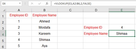 The VLOOKUP function will search for the value "1" inside the first column in the range A2:B6 in the following figure. It will find it and return the corresponding value in the second column, which is the name Ahmed. . 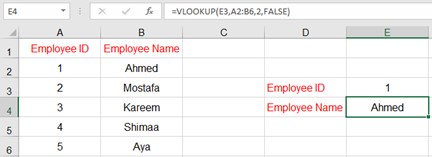VLOOKUP will search for the value "6" inside the first column in the range A2:B6 in the following figure. However, it will not find it. Therefore, it will not search for an approximate value and returns the error #N/A. The #N/A error appears when using the VLOOKUP function whenever it can't find the lookup value. Whenever you do a VLOOKUP and know you're looking up an existing value, it might be an issue with how your data was inputted in the table. Check out our tips and tricks video about cleaning up messy data!

Example of VLOOKUP to Find an Approximate Value

The following is a guide on how to calculate the estimate. It shows what is the corresponding sum for each forecast as follows:

• If the sum is greater than or equal to 0 and less than 50, the grade is Fail
• If the sum is greater than or equal to 50 and less than 65, the quality is acceptable
• If the sum is greater than or equal to 65 and less than 75, the quality is good
• If the sum is greater than or equal to 75 and less than 85, the quality is excellent
• If the sum is greater than or equal to 85 and less than or equal to 100, it is excellent

Accordingly, the parameters of the VLOOKUP function will be as follows:

• lookup_value: the value you want to search for, which is the value in cell E3
• table_array: the table (the range) containing the data, the range A2:B6. Note that the content does not include cell A1 and B1 addresses because we will not use them in the search. They are just addresses for data and not primary data.
• col_index_num: the order of the column containing the value returned by the function, which is column number 2
• [range_lookup]: We want to find an approximate value so that this parameter will take the value TRUE or 1

The VLOOKUP function will search for 65 in the first column in the range A2:B6 in the following figure. The estimate Goodwill finds and returns the corresponding value in the second column. 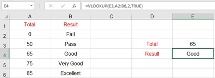The VLOOKUP function will search for the value 53 in the first column in the range A2:B6 in the following figure. It will not find it so it will search for the most considerable value smaller than the value 53. Then it will find the value 50 and return the corresponding value in the second column, which is the acceptable estimate. 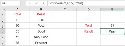If you've made it this far, I'm sure you can already imagine the plethora of possibilities in using VLOOKUP. Pair this with drop-down lists (which you can learn more about in this video), and you have a potent tool for your reports and dashboards. Lookup functions are the bread and butter of any dashboard. With the sheer amount of data that businesses, no matter how big or small, have, a quick and easy way to find values in a data table is a necessity. You can create employee databases with their ID numbers or order trackers using customer names or invoice numbers. In our Year Wise Analysis Template, you can see how the VLOOKUP function is combined with the IFERROR and nested in an IF function.

HOW TO USE VLOOKUP IN EXCEL: WALKTHROUGH

Use the Component Items and Supplier List tabs for this Excel VLOOKUP example. Let's say we're running a restaurant and placing weekly supplier orders. The chefs gave us a list of the required ingredients, and we needed to enter information about the supplier. There are three items we need to add to each order:

• Supplier name
• Supplier phone number
• Supplier delivery day

In this workbook, there are two tabs:

• Components Orders - This contains a list of component orders from our chefs.
• Supplier List - Contains information about suppliers, such as supplier name and phone number.

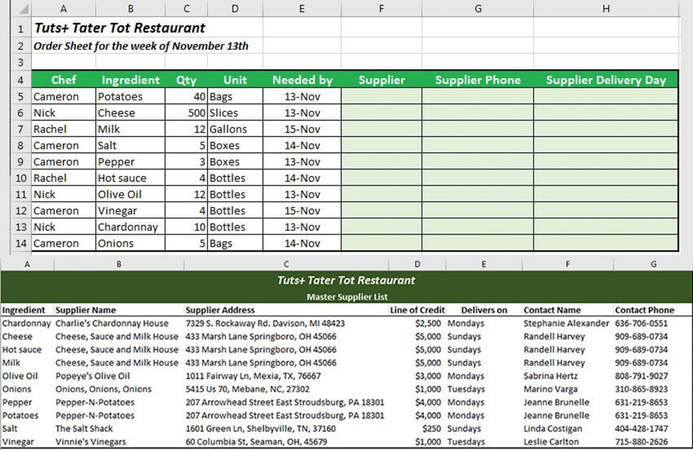  At the top, we have our order data on the Component Orders tab. Below is the Supplier List, which will serve as our search list. The legal field between the two tables is the Component tab.; let's use it to find the three areas and add them to the order list.

Step 1: Start Excel VLOOKUP Equation

On the Component Commands tab, click on the first empty cell, F5, then press the equal sign to start VLOOKUP. Then type "VLOOKUP (") to create the formula. =VLOOKUP( Remember that our primary key - the piece of data that appears in both lists - is an item, so we'll use it to search. First, either click on cell B5 or type it into the formula. Next, add a comma after "B5" to enter the next part of the formula. =VLOOKUP(B5 Now, give the formula of the search list. While the procedure is still open, click on the Supplier List tab. Start in the column in the range that contains the shared data. Now, click on cell A3, then click and drag to highlight and select A3 to G13, the entire lookup table. Press F4 on your keyboard to make the formula an absolute reference (more on this later). Finally, enter another comma. 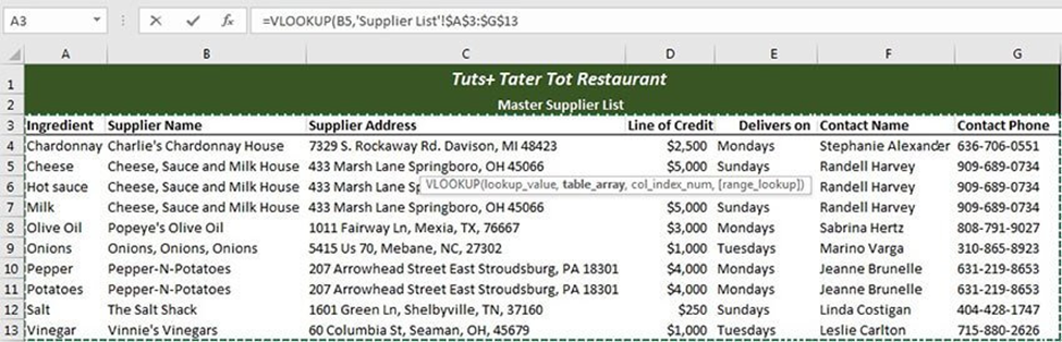Direct Excel to the search menu. After entering the comma for the search cell, switch tabs and direct Excel to the search menu. Next, click and drag between cells A3 and G3 to select the data to search. Be sure to press F4 on your keyboard during this step to create an absolute reference, which will lock cells for use in searching. The best part about this function is that it's one of the early versions of the lookup functions that Excel offers, so it's super accessible, and you can even do it on Google Sheets. If you want to see more great examples of how to get creative with nested VLOOKUPS, most of Simple Sheets' template dashboards use them. Why not skip making your own and sign up for FIVE FREE templates?