How to Compare Two Columns in Excel

A lot of entry-level jobs would have you doing simple data analysis tasks such as making you compare data and work with multiple columns, compare two columns in Excel, or compare multiple columns. That is why any young professional needs to master these skills to show everyone you're a wizard in the Sheets! You can use the essential tools that Microsoft Excel gives you. Tools like conditional formatting and data validation can significantly help you compare two columns or look out for missing data points to help point out different values or outliers in your data. These tools can also help see row differences in aligned data. Excel also has a bunch of near and straightforward formulas and functions that can aid you in this quest. The formula method is the bread and butter of many Excel users because of its versatility. Functions such as the EXACT and MATCH functions help you seek out mismatched data or identical entries and see if they're a full match. Pair these with an IF function, and then you've got the beginnings of a rad worksheet. The IF function allows you to run a logical test to see matching cells, which could be useful for row comparison. Other functions can also help you validate

Here are a Few Examples of How to Compare Two Columns in Excel Using a Simple Formula

Using the ISERROR Function and the MATCH Function

Suppose you have two tables of students' names in Column A and Column B of your Worksheet, and some of them are in two columns, but you want to compare these two columns and have only the differences appear in the other table. 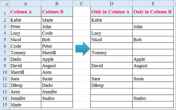To list unique values from the two lists separately, you can apply the following formulas:

1. Enter this formula in the first column of the second table, cell D2: =IF((ISERROR (MATCH(A2,$B$2:$B$14,0))), A2,"), (A2 is the first cell inside column A that you want to compare with column B and Range B2:B14 refers to another column you want to compare) and then press the Enter key:

2. Drag the fill handle down to the cells that you want to apply this formula, and all the unique values in column A are only inserted once: 3. Keep entering this formula: = IF ((ISERROR(MATCH(B2,$A$2:$15,0))),B2,"") into cell E2, and press Enter key: 4. Select cell E2, and drag the fill handle to the cells that you want to contain this formula, after which all the names in column B have been extracted only as follows: Now all the unique names in both columns are listed. Make sure not to drag down the formula until the last row because it will return a 0 value for the last one since Cell B15 is an empty string.

Compare Two Columns, Row by Row.

Below is a dataset where I need to check in the same row whether or not the names in column A match those in column B.

Comparing Columns by Row Position to Get an Exact Match

Usually, if you want to compare two cells belonging to a single row by row to look for matching values or get the same values, you can use the following formula: =B2=C2 Press the Enter key and drag the fill handle down to cell D8. If the formula returns TRUE, the two-column values are the same; if it returns FALSE, they are different. This method seeks out the same values and is case-insensitive.

Compare Two Cells in the Same Row for Exact Matches or Case Insensitive (Using the IF formula with EXACT Function)

If you want to compare two columns row by row in insensitive characters or get more descriptions such as match or mismatch, you can use the IF function alongside the EXACT Function to get the same values. We want to compare both columns for an exact match. If you want to use the text “Match” and “Mismatch” to describe the results of the comparison, please use the following formula: =IF (EXACT(B2, C2), “Match,” “Mismatch”) Press the Enter key to get the first result, then drag the AutoFill handle to cell D8. The formula will give you a Match if they are the same value and a Mismatch if not.

Compare Cells in the Same Row for a Case-Insensitive Match

If you want to compare cells that are not case-sensitive, you can use the formula below: =IF(B2=C2,"Match","Mismatch") Press the Enter key to get the first result, then drag the AutoFill handle to cell E8.

Compare Cells in the Same Row and Highlight Matching or Unmatched Data (Using Conditional Formatting)

Suppose you want to distinguish matching or different values. In that case, the Conditional Formatting feature can help you by allowing you to highlight cells and even highlight rows that will fit your conditional formatting parameters. This is a neat and fast way to highlight row differences without dealing with functions on your Worksheet.

1. Select the two columns used for comparison (B2: C8, excluding column headers), then click Home> Conditional Formatting> New Rule.

2. In the New Format Rule appeared dialog, click to use a formula to specify the cells to format in the Select a rule type, then type = $ B2 = $ C2 in the Format Values text box formula is correct. 3. Now, click a shape to display the Format Cells dialog, then under the Run tab, choose one color that you want to highlight matches. Or, you can change the font size, cell boundaries, or number format to beat matches as you want on other tabs. 4. Click OK> OK to close the dialog boxes; the cells in the same row will be selected if they are identical. If you want to highlight mismatch values, use this in File = $ B2 <> $ C2 in the textbox values format, where this formula is correct in the Edit Formatting Rule dialog. Then the differences between two columns in the same row will be highlighted with a specific color. Using the different methods above will give you a good idea that it's essential to consider how you construct your entire dataset. If you already know that you'll be needing to compare values, make sure that the data structure of your Worksheet is efficiently made so you can quickly call up all the values and be able to easily see the compared columns so you can make the most out of your entire data ranges.

Compare Two Columns Row by Row and Mark Mismatch Values (using VBA)

This tutorial is for you if you want to compare two columns row by row with VBA code.

1. Enable the Worksheet containing the two columns used for comparison, and press the ALT + F11 keys to enable the Microsoft Visual Basic for Applications window.
2. In the popping dialog, click Insert> Module.

Then copy and paste the macro below into the new module script.

• Sub ExtendOffice_HighlightColumnDifferences()
• 'UpdatebyKutools20201016
• Dim xRg As Range
• Dim xWs As Worksheet
• Dim xFI As Integer
• On Error Resume Next
• SRg:
• Set xRg = Application.InputBox("Select two columns:", "Kutools for Excel", , , , , , 8)
• If xRg Is Nothing, Then Exit Sub
• If Xorg.Columns.Count <> 2 Then
• MsgBox "Please select two columns"
• GoTo SRg
• End If
• Set xWs = xRg.Worksheet
• For xFI = 1 To xRg.Rows.Count
• If Not StrComp(xRg.Cells(xFI, 1), xRg.Cells(xFI, 2), vbBinaryCompare) = 0 Then
• Range(xRg.Cells(xFI, 1), xRg.Cells(xFI, 2)).Interior.ColorIndex = 7 '. You can change the color index as you need.
• End If
• Next xFI
• End Sub

Press the F5 key to run the code. Select the column against which you want to compare duplicate values in the first pop-up dialog. Click OK. In the second dialog box, select the column in which you want duplicate values highlighted.

• The code compares the columns with case sensitivity.
• In VBA, you can't exactly make use of the fill color icon, but you can change the shading color based on your unique need by changing the color index in the code, color index reference:

This method is more complicated than hitting that format button but also creates an excellent gateway into coding in Excel.