
4 Ways to Unhide Rows in Google Sheets
Feb 10, 2023
Unhidng rows in Google Sheets is a handy application that makes it easy for anyone to organize and manage their data within Google Sheets by offering a simple solution for hiding specific rows.
In this blog, we'll explore the following:
Get our free Excel formulas cheat sheet
Plus new tutorials and template drops. Enter your email and we'll send it over.
-
Four easy techniques to unhide rows in Google Sheets
-
Unhide Columns
-
Final Thoughts on How to Unhide Rows in Google Sheets
-
Frequently Asked Questions on How to Unhide Rows in Google Sheets
You can also watch the video below to see how it's done if you are more of a visual learner. Like & subscribe for more of the best spreadsheet tips!
Learn These 4 Easy Techniques to Unhide Rows in Google Sheets.
-
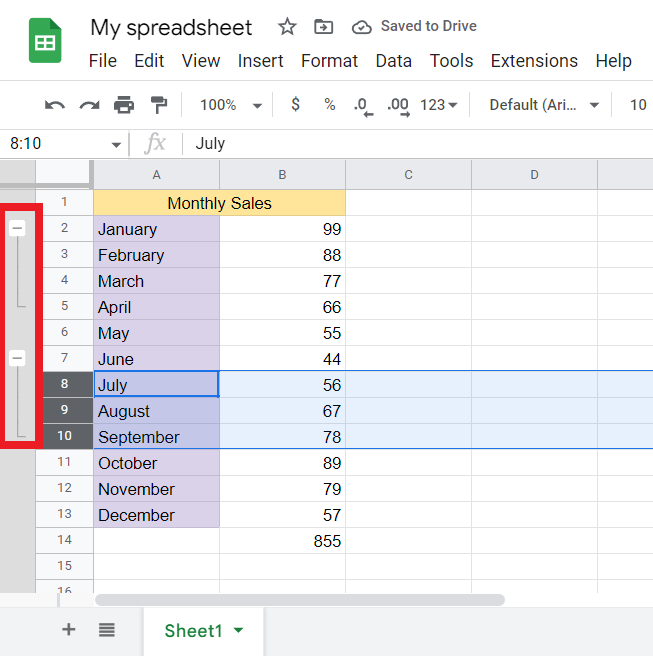
Unhide rows by clicking the upward/downward, pointing two arrows.
The rows from 3 to 8 are hidden on this spreadsheet. You can see that they are hidden because the numbering goes from 2 to 9, and there are two arrows next to the range of numbers.
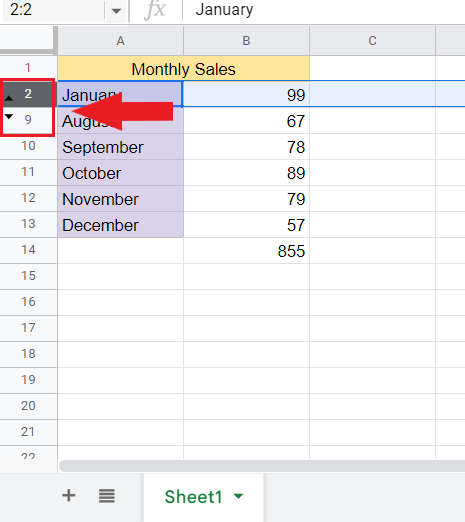
If you click the upside-down pointing arrows or the arrow bar, Google Sheets will show the data in the hidden rows again.
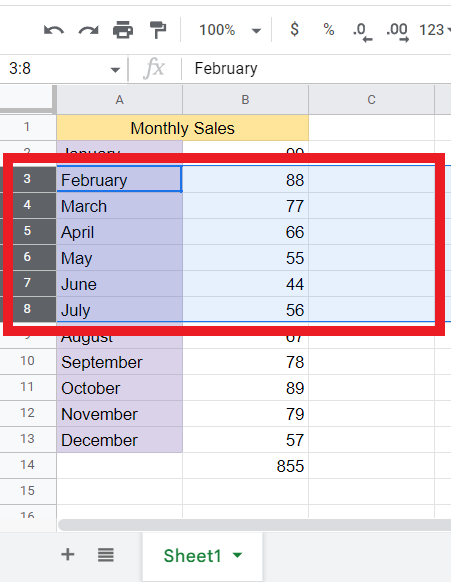
The highlighted rows are the missing rows which are multiple rows of 3 to 8, and you can also know it's one of the disappeared rows if there is a gray rectangle with the row number inside.
-
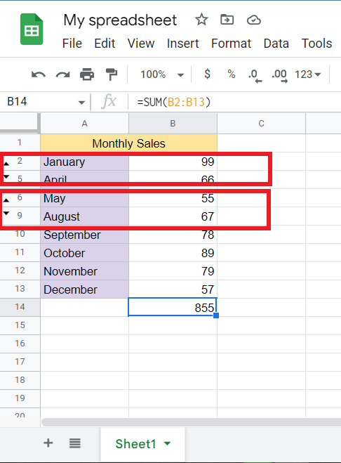
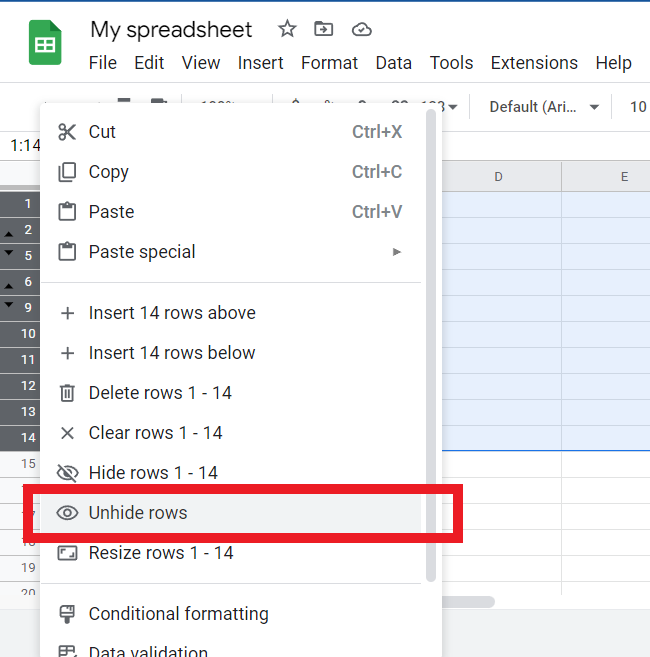
To unhide rows in a selection range, do the following:
The information in rows 3, 4, 7, and 8 is hidden. The upside-down arrows of the row numbers tell us which rows are hidden.
If we want to see the hidden information, we have to unhide the rows. We follow the same process to unhide two or more groups of hidden rows.
To select the range of rows you want to show, left-click on a row above the first hidden group.
While holding the shift key, click on a row below the hidden group range.
To find all the hidden rows, highlight the entire range of rows; if you want to select the whole sheet, press Ctrl+A on your keyboard.
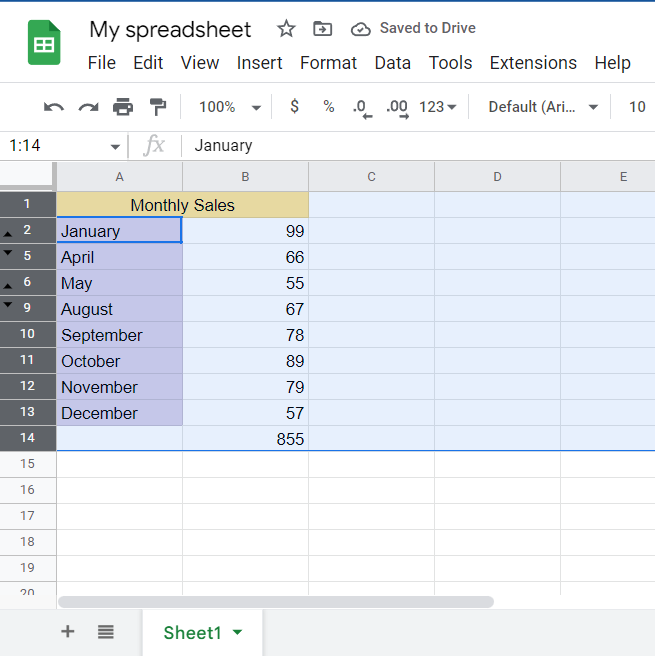
Click on the right side of your mouse within the selected range. A menu will pop up and show unhide rows option. Choose "Unhide rows." Or, you can use the critical shortcut Ctrl+Shift+9.
-
Unhide set groups rows in Google Sheets.
Google Sheets has a feature that lets you easily unhide rows, and the data won't disappear when you choose to unhide it. The "group" function assigns a "plus and minus" icon to a row range. This allows you to collapse or expand the rows within that range.
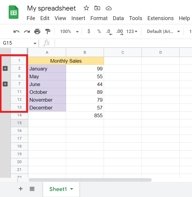
Click on the icon to show the hidden rows. If you're working on a shared spreadsheet with others, adding group-based hiding rows is an excellent way to keep the obscure row feature others added to the sheet while still being free to view content in hidden rows.
-
How to make filtered rows visible again in Google Sheets
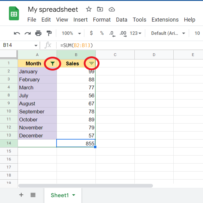
A filter is a way to hide some of the data. Check the rows if you can see rows 5, 6, and 7 on a spreadsheet.
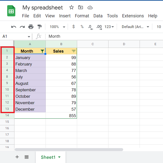
You can tell if a filter has been applied to data in your spreadsheet if you see the filter icon in each header row cell. For example, the filter icon indicates that filters are active.
You can turn off filters by going to the "Data" tab and selecting the "Turn off filter" choice.
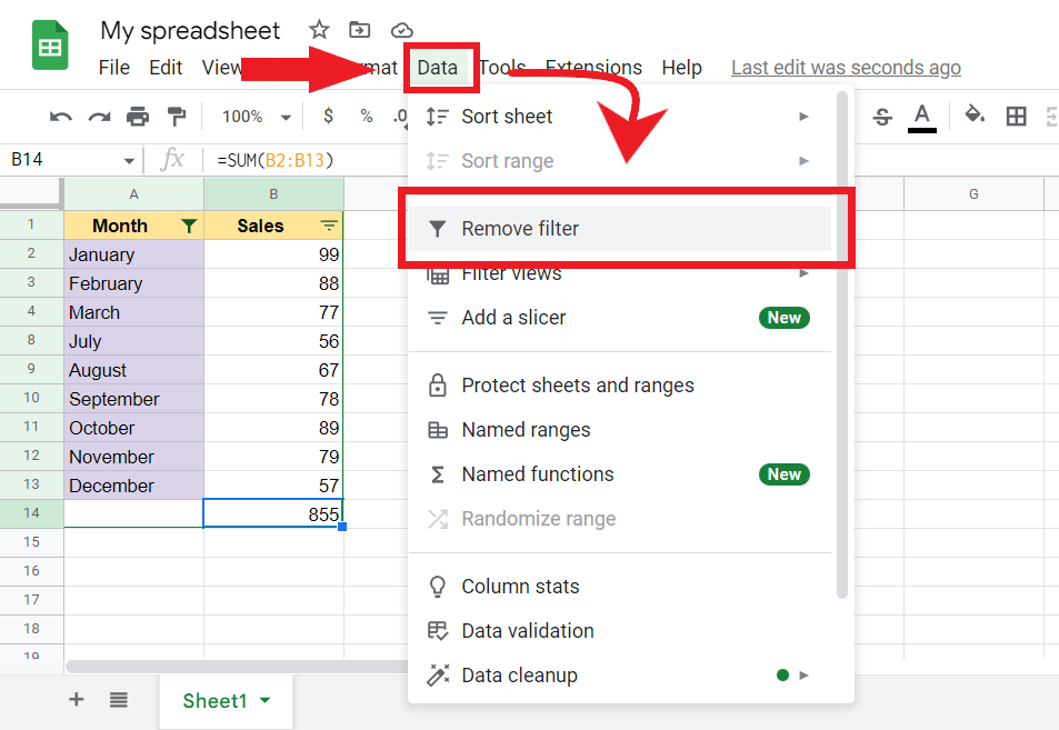
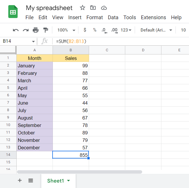
By removing filters, you can notice hidden rows in the sheet.

Unhide Columns.
To unhide columns, follow the same steps you would hide rows. This is a quick way to make your spreadsheets look neat and organized.
-
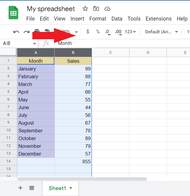
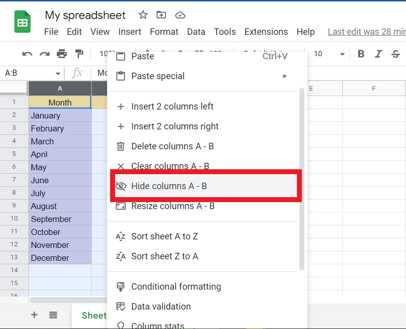
To create your data range, you'll need to select all of the relevant columns. Quickly achieve this by simply clicking and dragging across their corresponding letters!
-
Click on a column letter in the selected range. Right-click and select "Unhide columns" from the Menu.
Read Also: The Top 5 Google Sheets Formulas You Need to Know
Final Thoughts on how to Unhide Rows in Google Sheets.
Unhiding rows can help you save time and effort scanning your worksheets and improve your skills using Google Sheets!
You can visit our homepage for more easy-to-follow how-to and step-by-step guides. Check the links in related articles for further details about Excel Templates!
Frequently Asked Questions on How to Unhide Rows in Google Sheets:
How do I unhide rows in Google Sheets?
You must select the rows directly below and above the hidden one, right-click with your mouse, and click "Unhide Rows."
How do I view hidden rows in Google Sheets?
To make the rows visible, select 'View' from the Menu and click 'Unhide Rows.'
How do I unhide multiple rows in Google Sheets?
Highlight the rows that are hidden. Then select "Unhide" from the toolbar menu. This will make the hidden rows appear again so you can keep working.

Related Articles:
How to Unhide All Rows in Excel: A Step-by-Step Guide
Want to Make Excel Work for You? Try out 5 Amazing Excel Templates & 5 Unique Lessons
We hate SPAM. We will never sell your information, for any reason.

