Beginners Guide: How To Compare Two Excel Sheets For Matching Data
Mar 15, 2023
To compare two Excel sheets for matches, put both sheets in the same workbook, add a helper column next to your first list, and enter =IF(ISNUMBER(MATCH(B2,Sheet1!$B$2:$B$6,0)),"Match","No match"). Fill it down. Every row now says whether that value exists on the other sheet. Lock the lookup range with dollar signs or the results will be wrong.
Comparing two spreadsheets by eye is slow and unreliable. This guide covers five ways to cross reference two Excel sheets and find the values they have in common, from a one-formula helper column to a Power Query merge, plus what to do when two values look identical on screen and Excel still says they do not match.
Get our free Excel formulas cheat sheet
Plus new tutorials and template drops. Enter your email and we'll send it over.
Last updated: August 23, 2026
What this guide covers
- Can you cross reference two Excel sheets?
- Method 1: MATCH, the fastest helper column
- Method 2: Highlight the matches with conditional formatting
- Method 3: VLOOKUP to pull the matching row across
- Method 4: XLOOKUP, the modern replacement
- Method 5: COUNTIF to count matches instead of finding them
- Bonus: Power Query for large lists
- Which method should you use?
- Why does Excel say no match when the values look identical?
- Matches or differences? They are different jobs
- Frequently asked questions
Read Also: How to compare two Excel files or sheets for differences
Can You Cross Reference Two Excel Sheets?
Yes. Excel has no single "compare sheets" button for this, but cross referencing two sheets is a standard job and any of the five methods below does it in a couple of minutes. Nothing needs installing and nothing needs a subscription.
Two things make it much easier, and both are worth doing before you start:
- Put both sheets in the same workbook. You can reference another workbook, but the formula gets long and it breaks the moment that file moves or is renamed. If your data is in two separate files, right-click a sheet tab, choose Move or Copy, and copy it into the other workbook first.
- Decide which column is the key. Cross referencing works on one column of unique-ish values: an ID, an email address, an order number, a name. Everything else is just data that travels with it.
The rule to remember: matching is a one-column job. If you find yourself trying to compare six columns at once, you are usually looking for differences, which is a different task with a different tool. There is a section on that below.
Method 1: MATCH, the Fastest Helper Column
This is the quickest way to compare two Excel sheets for matches. It adds one column that says, for every row, whether that value also exists on the other sheet.
-
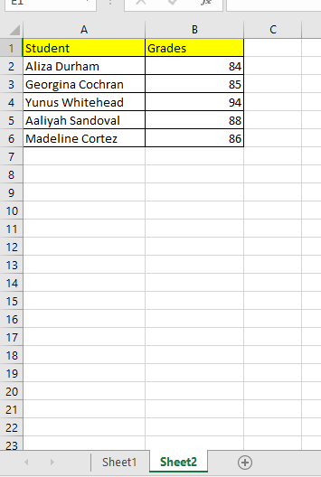
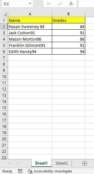
Prepare your two worksheets in the same workbook.
-
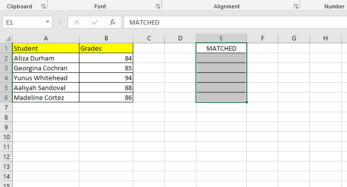
Select an empty column next to your list. This is your helper column.
-
Enter the MATCH formula, pointing at the column on the other sheet:
=MATCH(B2,Sheet1!$B$2:$B$6,0)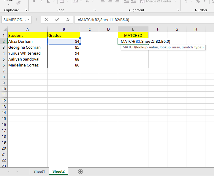
-
Press Enter, then fill the formula down the column.

Reading the result: a number means the value was found, and the number is the row position it was found at. #N/A means it was not found on the other sheet. So a column of numbers with a few #N/A values is exactly what you want to see.
The most important detail on this page: the dollar signs in $B$2:$B$6 are not optional. They lock the lookup range so it stays put when you fill down. Without them, row 3 searches B3:B7, row 4 searches B4:B8, and every result below the first row is wrong. If your matches look randomly missing, this is almost always why.
To get words instead of numbers, wrap it in IF and ISNUMBER:
=IF(ISNUMBER(MATCH(B2,Sheet1!$B$2:$B$6,0)),"Match","No match")
The third argument of MATCH, the 0, means exact match. Leave it out and Excel does an approximate match on data it assumes is sorted, which quietly returns wrong answers on unsorted lists.
Method 2: Highlight the Matches with Conditional Formatting
Formulas tell you the answer. Colour shows you the answer. Use this when someone else has to read the result.
-
Add the helper column from Method 1 so each row reads "Match" or "No match".
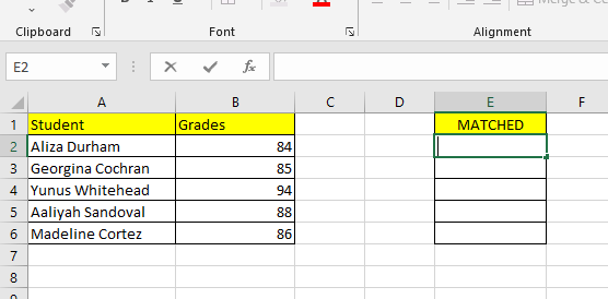
-
Enter the formula and confirm it returns text rather than an error:
=IF(ISNUMBER(MATCH(B2,Sheet1!$B$2:$B$6,0)),"Match","No match")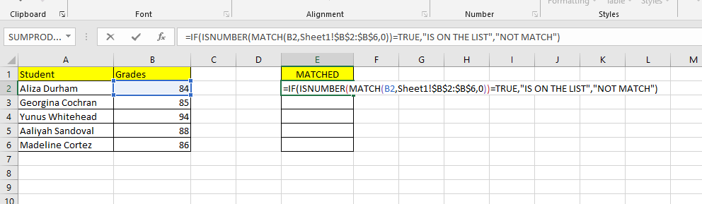
-
Press Enter, then use the Fill Handle to drag it down the column.
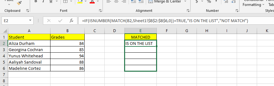
-
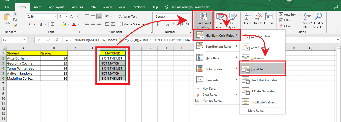
Select the helper column, then go to Home > Conditional Formatting > Highlight Cells Rules > Equal To.
-
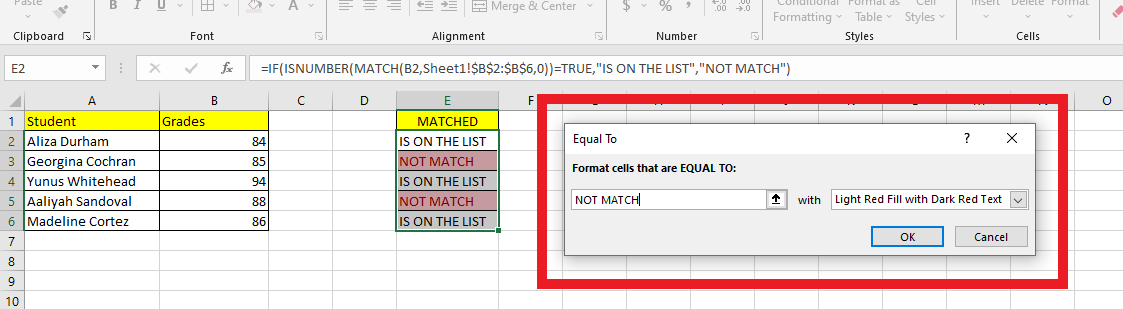
Type Match in the box and pick a fill colour.
-
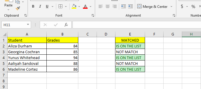
Click OK. Every row that exists on both sheets is now highlighted.
To highlight the data itself rather than the helper column, select your whole data range, choose Conditional Formatting > New Rule > Use a formula to determine which cells to format, and enter:
=COUNTIF(Sheet1!$B$2:$B$6,$B2)>0
Note the mixed reference $B2: the column is locked, the row is not. That is what makes the rule colour the entire row based on the value in column B.
Method 3: VLOOKUP To Pull the Matching Row Across
MATCH tells you whether a value exists on the other sheet. VLOOKUP brings the matching information back with it, which is usually what you actually want.
- In your helper column, enter
=VLOOKUP(B2,Sheet1!$B$2:$D$6,3,FALSE). B2is the value you are looking for.Sheet1!$B$2:$D$6is the table on the other sheet.3is which column of that table to return, counting from the left of the range.FALSEforces an exact match.- Fill down. Rows that exist on both sheets bring their data across. Rows that do not return
#N/A. - To hide the errors, wrap it:
=IFERROR(VLOOKUP(B2,Sheet1!$B$2:$D$6,3,FALSE),"Not found").
The VLOOKUP trap that catches everyone: the lookup value must be in the first column of the range you give it. $B$2:$D$6 looks up in column B, so it can return C or D but never A. If the value you need is to the left of your key, VLOOKUP cannot do it. Use XLOOKUP or INDEX MATCH instead.
Method 4: XLOOKUP, the Modern Replacement
XLOOKUP does the same job as VLOOKUP with fewer ways to get it wrong. It is available in Microsoft 365, Excel 2021, Excel 2024 and Excel for the web. It is not in Excel 2019 or earlier, so use Method 3 if you are on an older version.
- Enter
=XLOOKUP(B2,Sheet1!$B$2:$B$6,Sheet1!$D$2:$D$6,"Not found"). - The arguments read plainly: what to look for, where to look for it, what to return, and what to say if nothing is found.
- Fill down.
Why it is worth switching: XLOOKUP takes the lookup column and the return column separately, so the return column can sit anywhere, including to the left. It defaults to exact match, so there is no FALSE to forget. It has a built-in not-found argument, so you do not need IFERROR. And it does not break when someone inserts a column, because it is not counting positions.
Quotable rule: VLOOKUP counts columns, XLOOKUP names them. That single difference is why VLOOKUP formulas break when a colleague inserts a column and XLOOKUP formulas do not.
Method 5: COUNTIF To Count Matches Instead of Finding Them
Use COUNTIF when you care how many times a value appears on the other sheet, not just whether it appears at all. This is the right tool for finding duplicates across two lists.
- Enter
=COUNTIF(Sheet1!$B$2:$B$6,B2)in your helper column and fill down. - 0 means the value is only on this sheet. 1 means it appears once on the other sheet. 2 or more means the other sheet has duplicates of it.
- To flag only the duplicates, use
=IF(COUNTIF(Sheet1!$B$2:$B$6,B2)>1,"Duplicate","").
Worth knowing: COUNTIF never returns #N/A. It returns 0. That makes it easier to filter and sort than MATCH, and it is why COUNTIF is usually the better choice inside a conditional formatting rule.
One real limitation: COUNTIF treats text that looks like a number as a number. If your key column holds product codes such as "00123" and "123", COUNTIF may report them as the same thing. When the key is a code with leading zeros, use =SUMPRODUCT(--EXACT(Sheet1!$B$2:$B$6,B2)) instead, which compares strictly and is also case sensitive.
Bonus: Power Query for Large Lists
Formulas slow down on tens of thousands of rows. Power Query does the same comparison without adding a single formula to the sheet, and it refreshes with one click when the data changes.
- Click inside your first list and press Ctrl + T to make it a Table. Do the same on the second sheet.
- With the first Table selected, go to Data > From Table/Range. In the Power Query Editor, choose Close & Load To and select Only Create Connection. Repeat for the second Table.
- Go to Data > Get Data > Combine Queries > Merge.
- Pick your two queries, click the key column in each so both highlight, and set the Join Kind.
- Choose Inner to keep only rows that exist in both, which is your list of matches. Choose Left Anti to keep only rows that exist in the first list and not the second.
- Click OK, then Close & Load to drop the result onto a new sheet.
The payoff: when either source list changes, click Data > Refresh All and the comparison redoes itself. A formula-based comparison has to be rebuilt every time the ranges change size.
Which Method Should You Use?
| What you need | Use | Returns |
|---|---|---|
| Just tell me if this value is on the other sheet | MATCH (Method 1) | A position number, or #N/A |
| Show me the matches visually | Conditional formatting (Method 2) | Coloured rows |
| Bring the matching data across with it | VLOOKUP (Method 3) | The value from the chosen column |
| Same, but on Microsoft 365 or Excel 2021 and later | XLOOKUP (Method 4) | The value, and it will not break on inserted columns |
| How many times does this appear on the other sheet | COUNTIF (Method 5) | A count, 0 if absent |
| Codes with leading zeros, or case matters | SUMPRODUCT with EXACT | A strict count |
| Tens of thousands of rows, or a comparison you repeat | Power Query merge | A refreshable table of matches |
| Which cells changed between two versions of a file | Not this page. See the differences guide | A cell-by-cell diff |
Why Does Excel Say No Match When the Values Look Identical?
This is the single most common problem with cross referencing, and it is almost never a formula fault. Excel is comparing something you cannot see on screen.
| Cause | How to spot it | Fix |
|---|---|---|
| Trailing or leading spaces | =LEN(B2) returns more characters than you can count |
Wrap the lookup value: =MATCH(TRIM(B2),...), or clean the column with TRIM and paste back as values |
| Numbers stored as text | Values sit left-aligned instead of right-aligned, or a green triangle appears | Select the column, click the warning icon and choose Convert to Number, or use Data, Text to Columns and finish |
| The lookup range is not locked | The first row matches and the rest fail | Add dollar signs: $B$2:$B$6 |
| Non-breaking spaces from a web or PDF paste | TRIM does not fix it | =SUBSTITUTE(B2,CHAR(160),"") before matching |
| MATCH is doing an approximate match | Results are wrong rather than missing | Add the third argument: MATCH(B2,range,0) |
| Dates that are really text | One column right-aligns, the other left-aligns | Convert both to real dates, then compare |
| Hidden characters or line breaks | =CLEAN(B2) changes the length |
Wrap the value in CLEAN as well as TRIM |
The fastest diagnostic: put =EXACT(A1,B1) beside two values you believe are the same. If it returns FALSE while your eyes say TRUE, the difference is whitespace, character encoding or a text-versus-number mismatch. Then run =LEN() on both to see which one is longer.
If the formula itself is not calculating at all, that is a different problem. See Excel formulas not calculating.
Matches or Differences? They Are Different Jobs
People search for both with almost the same words, and the tools are not interchangeable.
- Finding matches means comparing one key column across two lists to see which values appear on both. That is this page. MATCH, VLOOKUP, XLOOKUP, COUNTIF and a Power Query inner join all do it.
- Finding differences means comparing two versions of the same sheet cell by cell to see what changed. That needs a different approach, and we cover it in how to compare two Excel sheets for differences.
- Matching data across two sheets and merging it is a third job again, covered in how to match data from two Excel sheets.
- Comparing two columns on the same sheet is simpler than any of these. See how to compare two columns in Excel.
Microsoft's own reference for the function at the centre of all this is the MATCH function documentation, which is worth a look for the wildcard behaviour that most tutorials skip.
Read Also: Differentiate Between the Workbook and Worksheet in Excel?
Final Thoughts
Cross referencing two Excel sheets for matches comes down to one decision: do you want to know whether a value is on the other sheet, or do you want to bring its data across? MATCH and COUNTIF answer the first. VLOOKUP and XLOOKUP answer the second. Power Query answers both at scale.
Whichever you pick, lock the lookup range with dollar signs and force an exact match. Those two habits prevent most of the wrong answers people get from a comparison that looked like it worked.
Get more step-by-step Excel tutorials by visiting Simple Sheets! Check out the related articles below and our Facebook Page for Excel and Google Sheets templates!
Frequently Asked Questions
Can you cross reference two Excel sheets?
Yes. There is no single compare button, but a MATCH, VLOOKUP, XLOOKUP or COUNTIF formula in a helper column cross references two sheets in a couple of minutes. Put both sheets in the same workbook first, pick one key column such as an ID or an email address, and lock the lookup range with dollar signs.
How do I compare two Excel sheets for matches without a formula?
Use Power Query. Turn each list into a Table with Ctrl + T, load each as a connection-only query, then use Data, Get Data, Combine Queries, Merge and choose the Inner join kind. The result is a table containing only the rows that exist in both lists, and it refreshes with Data, Refresh All when the source changes.
Can I use INDEX MATCH across different sheets?
Yes. INDEX MATCH works across sheets exactly like VLOOKUP, and unlike VLOOKUP it can return a column to the left of the key. The pattern is INDEX with the column you want returned, then MATCH with the key and the column to search, both prefixed with the sheet name. On Microsoft 365 or Excel 2021 and later, XLOOKUP does the same thing in one shorter function.
Can I use VLOOKUP to compare two sheets?
Yes, with one constraint. VLOOKUP requires the value you are looking up to sit in the first column of the range you hand it, and it counts the return column by position. If the data you need is to the left of your key, or if someone might insert a column later, use XLOOKUP or INDEX MATCH instead. You do not need to name a range first, contrary to a lot of advice: a plain sheet reference such as Sheet1!$B$2:$D$6 works fine.
Why does MATCH return #N/A when both values look the same?
Almost always because the two values are not actually identical. Trailing spaces, numbers stored as text, and non-breaking spaces pasted in from a website are the three usual causes. Test it with =EXACT(A1,B1). If that returns FALSE while the cells look identical, wrap your lookup value in TRIM and CLEAN, or fix the column with Text to Columns.
What is the difference between comparing sheets for matches and for differences?
Matching compares one key column across two lists to find values that appear on both, which is what this guide covers. Finding differences compares two versions of the same sheet cell by cell to see what changed. They need different tools, so decide which one you actually want before you start.
Related Articles:
How to Compare Two Excel Sheets for Differences
How to Match Data from Two Excel Sheets in 3 Easy Methods
How to Compare Two Columns in Excel
XLOOKUP vs. VLOOKUP: Which is the Better Function?
Want to Make Excel Work for You? Try out 5 Amazing Excel Templates & 5 Unique Lessons
We hate SPAM. We will never sell your information, for any reason.