How to Make Negative Numbers Show Up in #Red in Excel

Microsoft Excel (for the most part) saves us a lot of time and trouble as it offers innovative and more accurate solutions regarding tables and calculations. These features make your work in Excel much more productive. Suppose you work as an accountant for a company, or if you have a small business that uses Excel, a bunch of numbers placed next to each other is a little challenging to navigate. More so, if you need to search specific values, over time, you may realize that searching multiple negative numbers in an Excel worksheet is challenging just by browsing the Excel worksheet category list. This causes many problems related to the accuracy of the calculations, as well as wasting time, is pretty distracting, and sometimes gives you overlapping numbers. Fortunately, we can mark all negative numbers in red using custom number formatting on the selected cells or make the numbers red using Excel's built-in tool, Conditional Formatting. These methods allow you to create your conditions, but in this article, we'll highlight negative numbers in red in Excel. We'll show you later in this post how to add the negative sign in the cell next to the negative value to be more precise and evident once you see it on the worksheet. Review the guidelines for customizing a number format number. With this method, negative numbers will be highlighted in the current worksheet. Just follow the next few steps, and you'll find that this is the shortest way to reach your goal of making negative numbers look red in parentheses with the negative sign. So, let's show you how to Make Negative Numbers Red in Excel:

How Do I Make Negative Numbers Appear in Parentheses

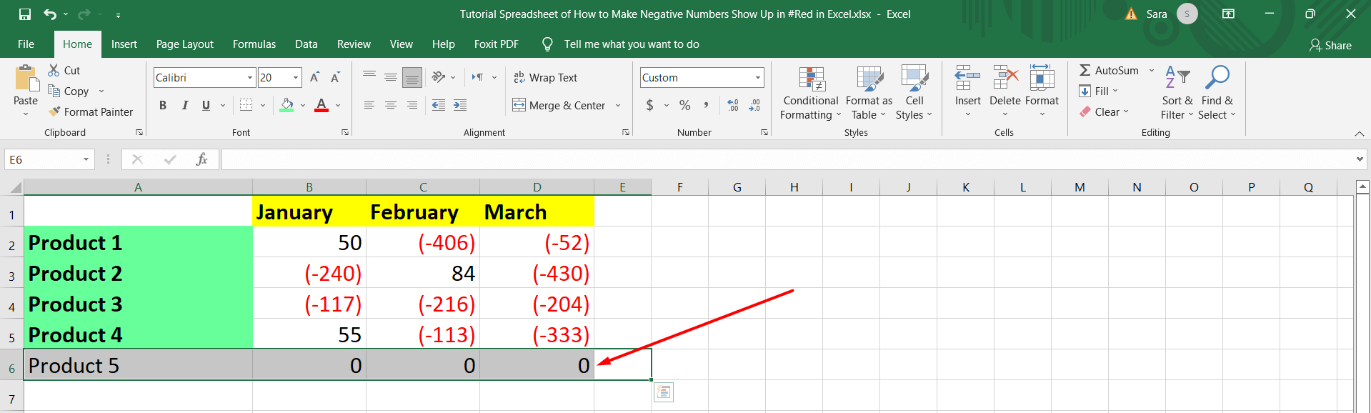
Now, we will show you how to bracket negative numbers in the Excel worksheet by custom number formats to make your work more professional using minimal effort. You can also use the attached MS Excel file to which the steps have been applied. For more practice, open the attached Excel file to create your file. Download the Tutorial Spreadsheet on How to Make Negative Values Show Up in #Red in Excel. This example shows a file containing the profits and losses of selling some products over several months. The negative numbers are losses, and the positive numbers are profits. You will also find a cell number format containing the number (0) that indicates the products that have not been sold over the months. We will also explain how to show the sign (-) instead of the number (0) in the format cells. Look at how to do it in the following steps found in the screenshots below: Step One: In the beginning, please Select all the cells in the workbook by highlighting them by clicking on the arrow on the top left side of the file. You will find it indicated by the red arrow in the screenshot below. 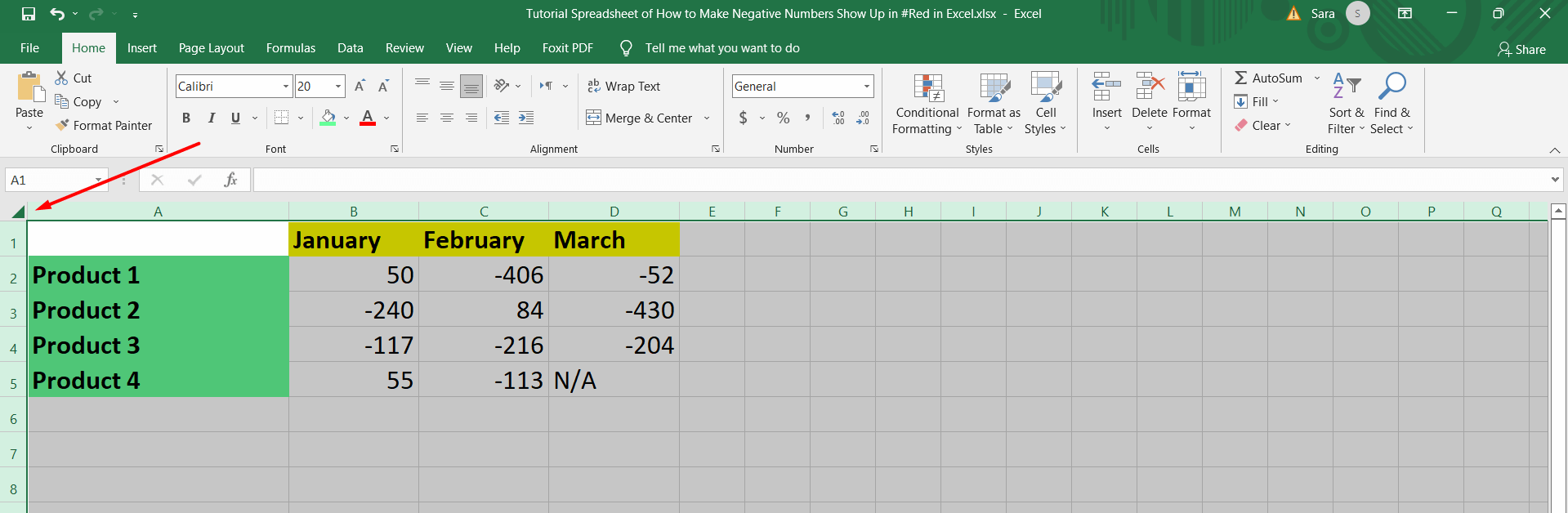Step Two: Click the right button on the mouse. A dialog box will appear; select the Format Cells dialog box option. As shown below. 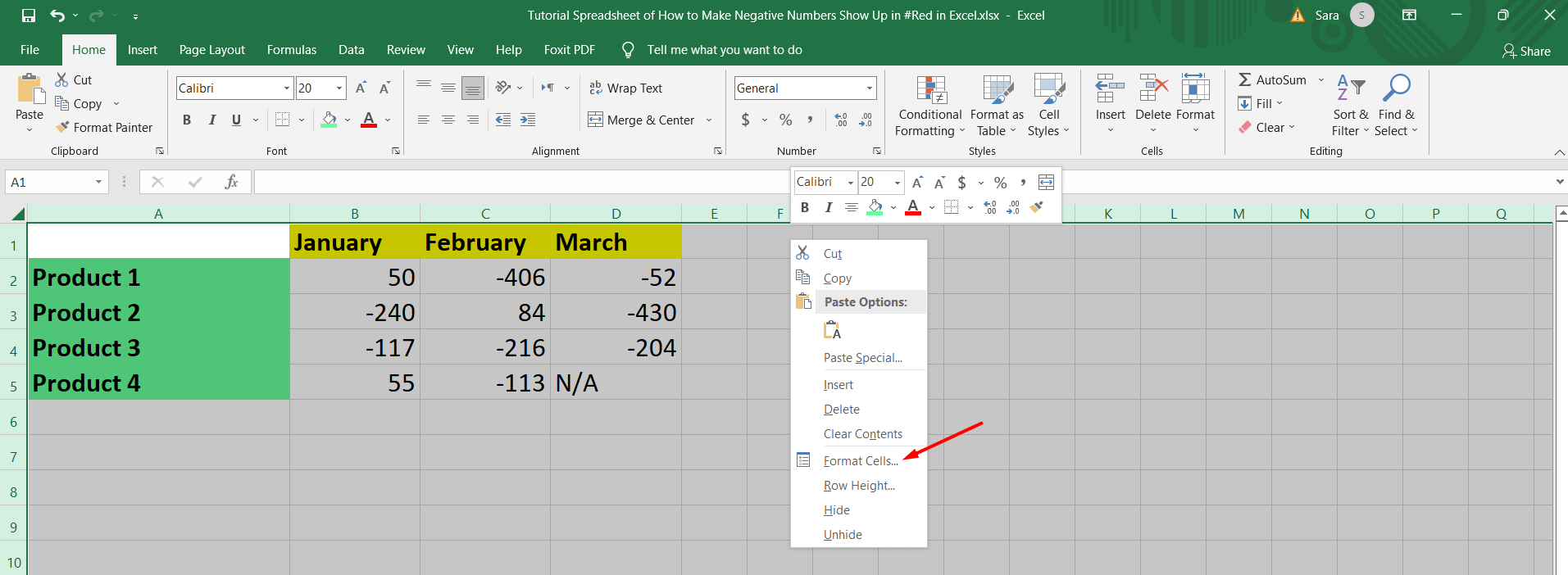Step Three: It will open a new window. Select the Custom Format option. 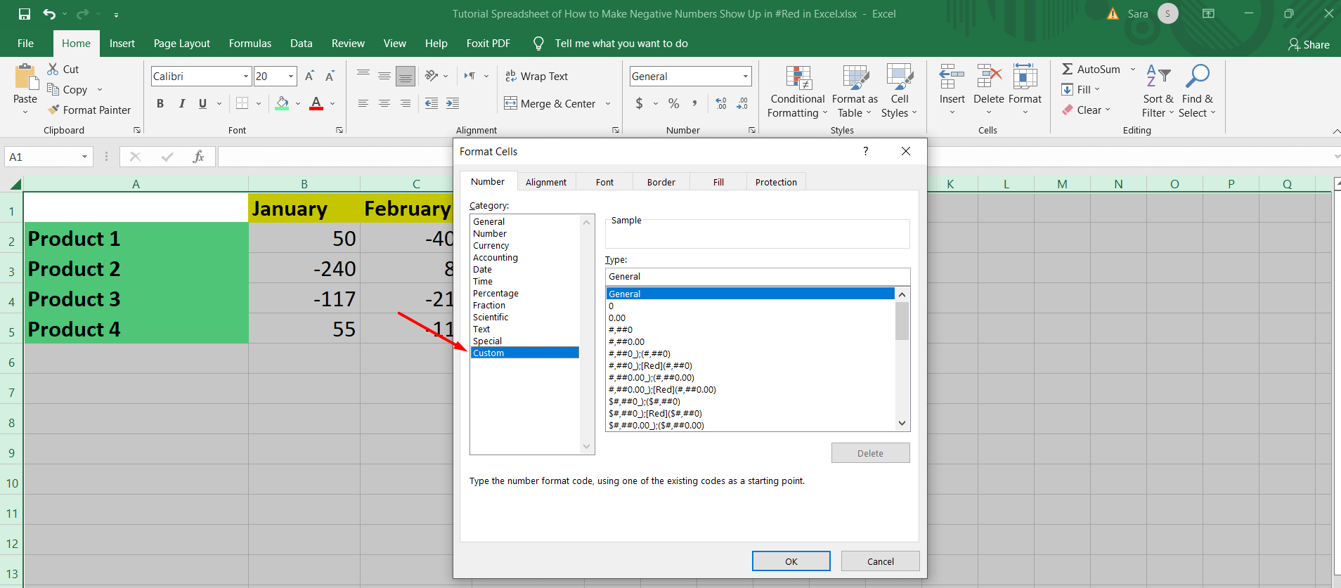Step Four: You will see the word "General" in the place indicated by the red arrow, as shown in the screenshot below. 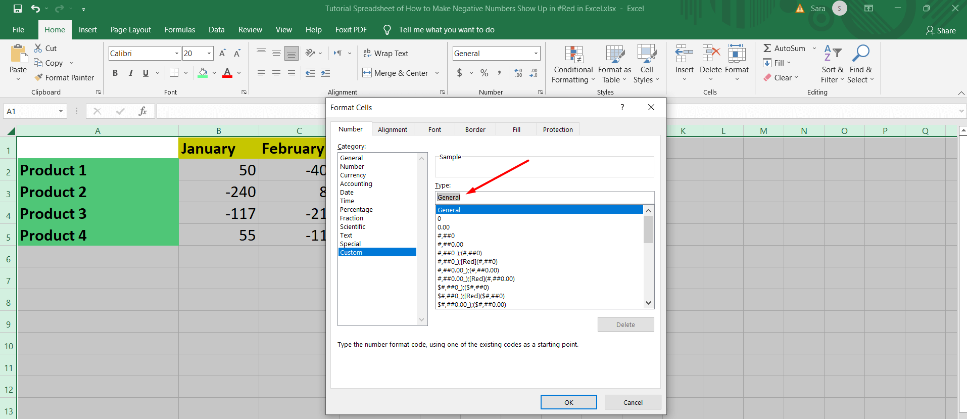Step Five: Copy the word "General" and paste it twice more to make it three terms in the format, separated by a decimal point without any space. Or, create/write this Excel formula: General; General; General. Or, You can find the exact format as the last option of the drop-down list.

Note:

The first "General" represents the format of the numbers if they are positive numbers. The second "General" represents the format of the numbers if they are negative. The third, "General," represents the format of the numbers if the number they are Zeros (0). 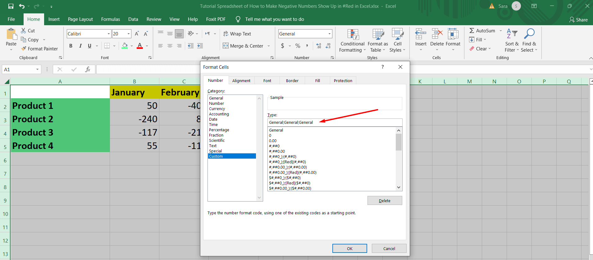Step Six: Now, choose the "Custom Format" and then put the second "General" for the number format of all the negative numbers bracketed. Or, write the formula like this: General;(General); General

Note:

You should add the brackets between the two decimal points left and right. 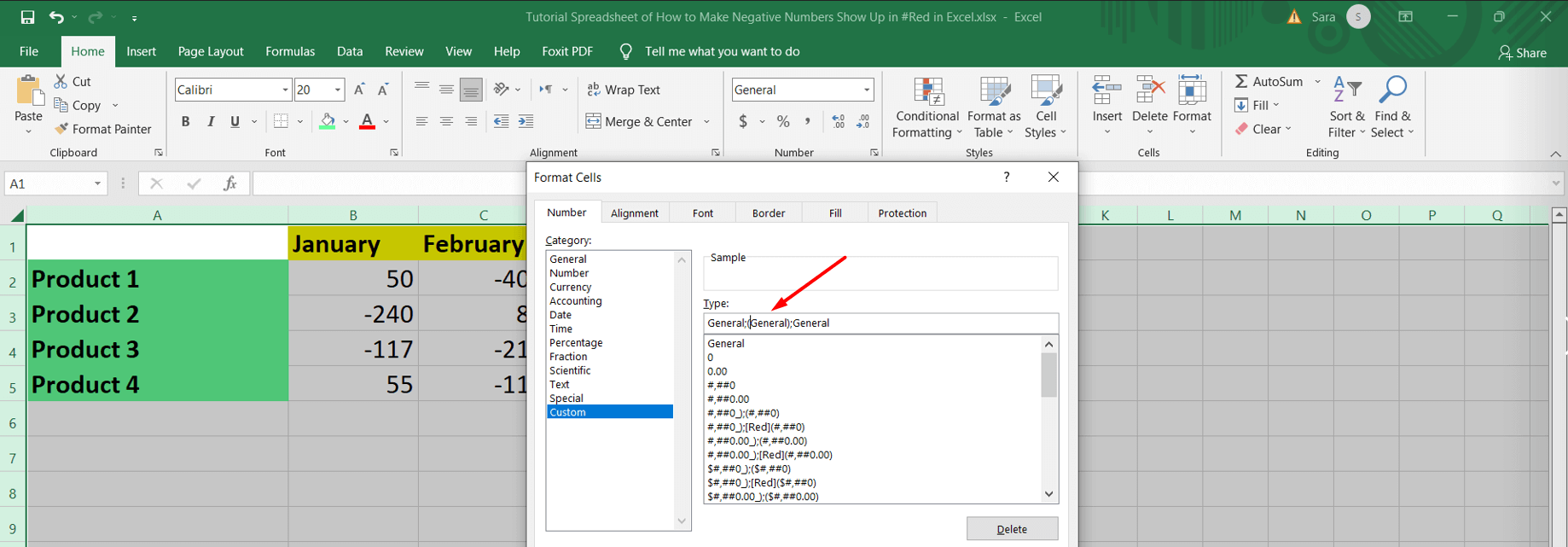Step Seven: Finally, save the formatting by pressing the OK button. 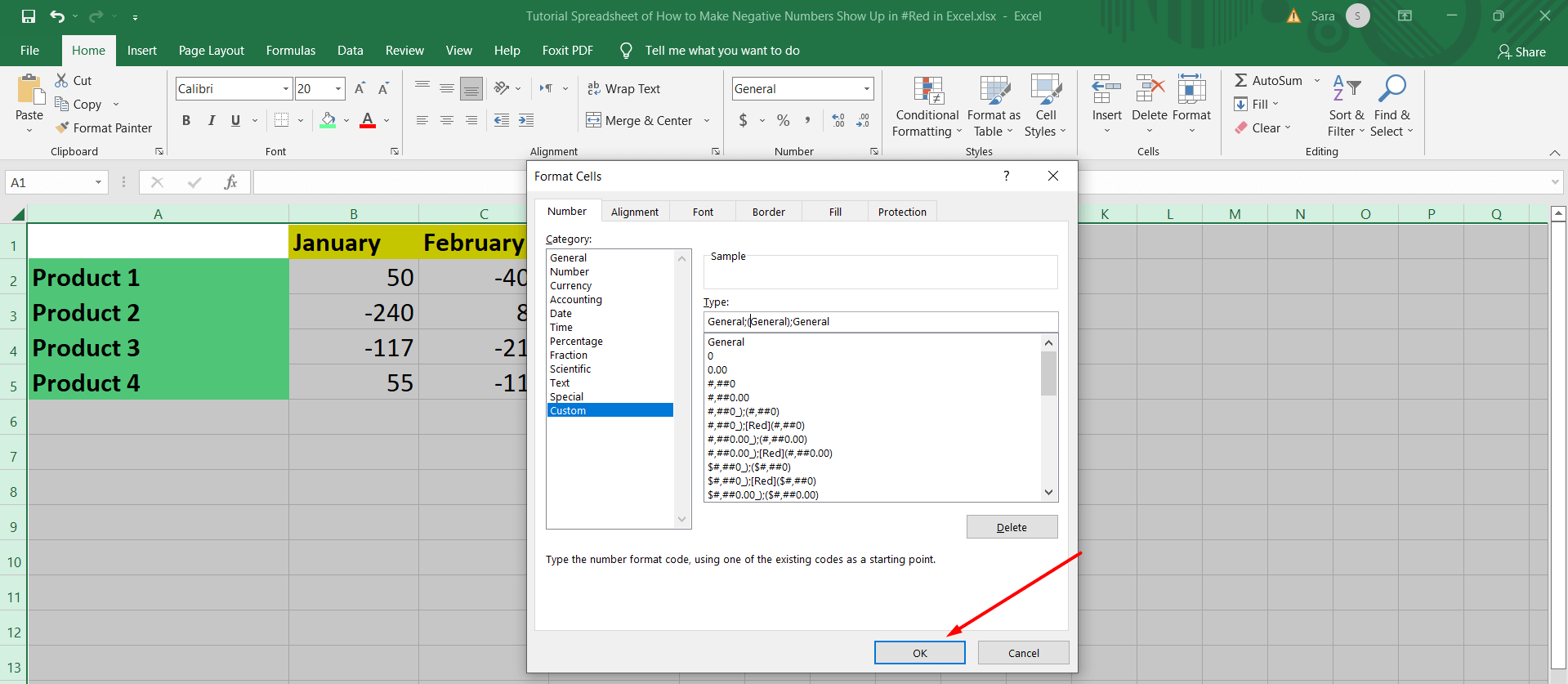Now, this displays negative numbers format as shown below.

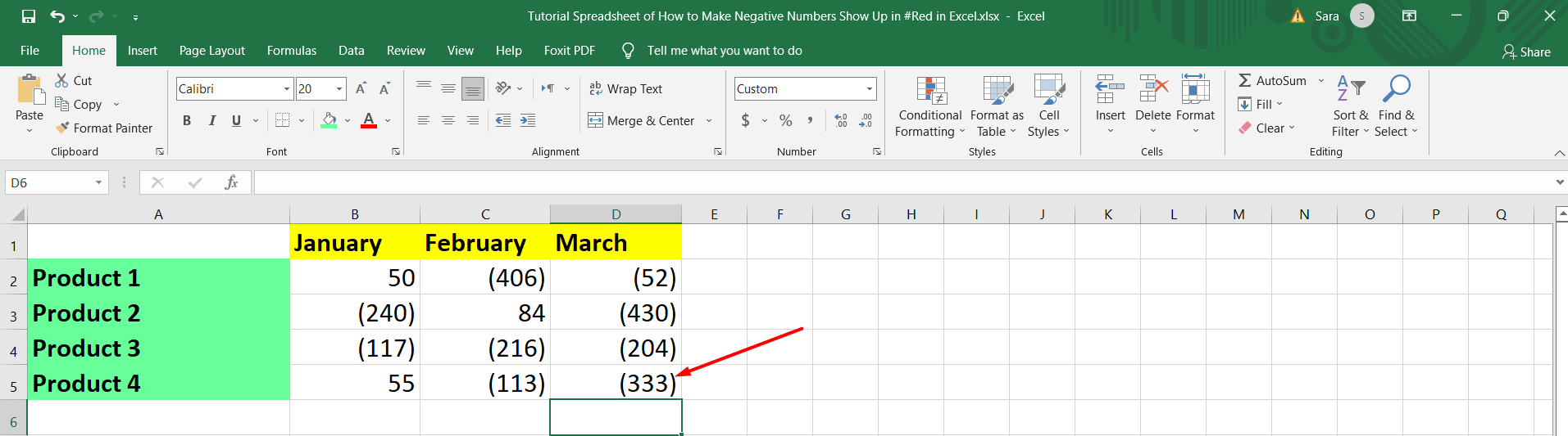
How Do I Make Negative Numbers In Red Color

In this post, also, by this new rule, you can change the font color of the minus numbers formatted to red. Make all the negative numbers dark red text. Apply the following formatting instructions to display negative numbers in red and keep the positive ones in the default color. Step One: Please select all the cells in the workbook by highlighting them by clicking on the arrow on the top left side of the file. You will find it indicated by the red arrow in the screenshot below. 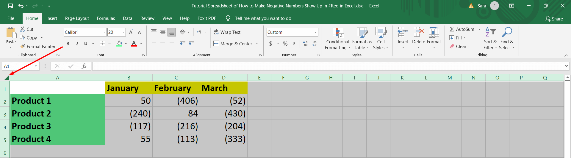Step Two: Click the right button on the mouse. A dialog box will appear; select the Format Cells dialog box option. As shown below. 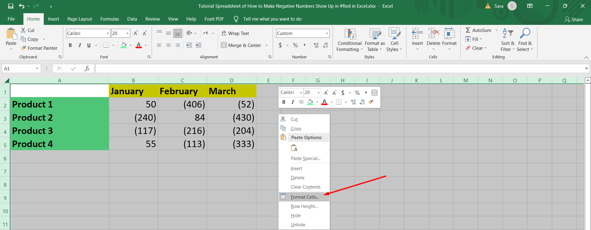Step Three: Choose the "Custom Format," and then you can add a "red" entry between these brackets "[]." Or, copy the following formula and paste it there: General;[red](General); General 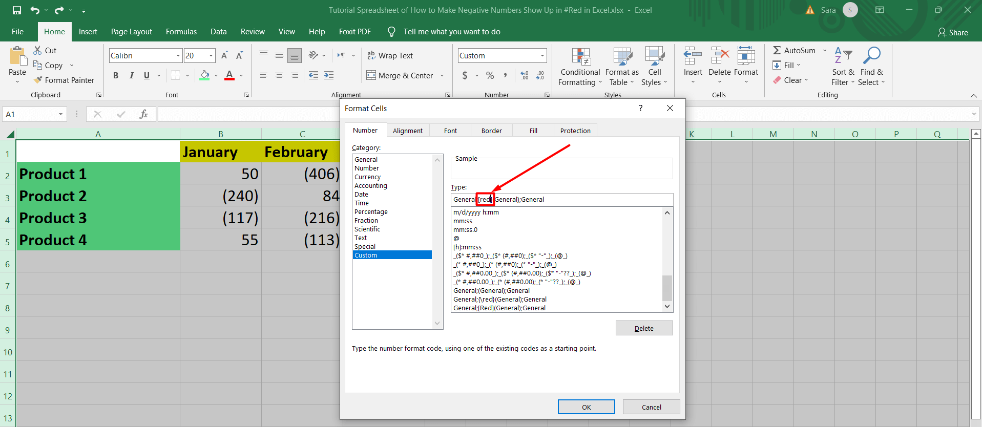Step Four: Finally, save the formatting by pressing the OK button. 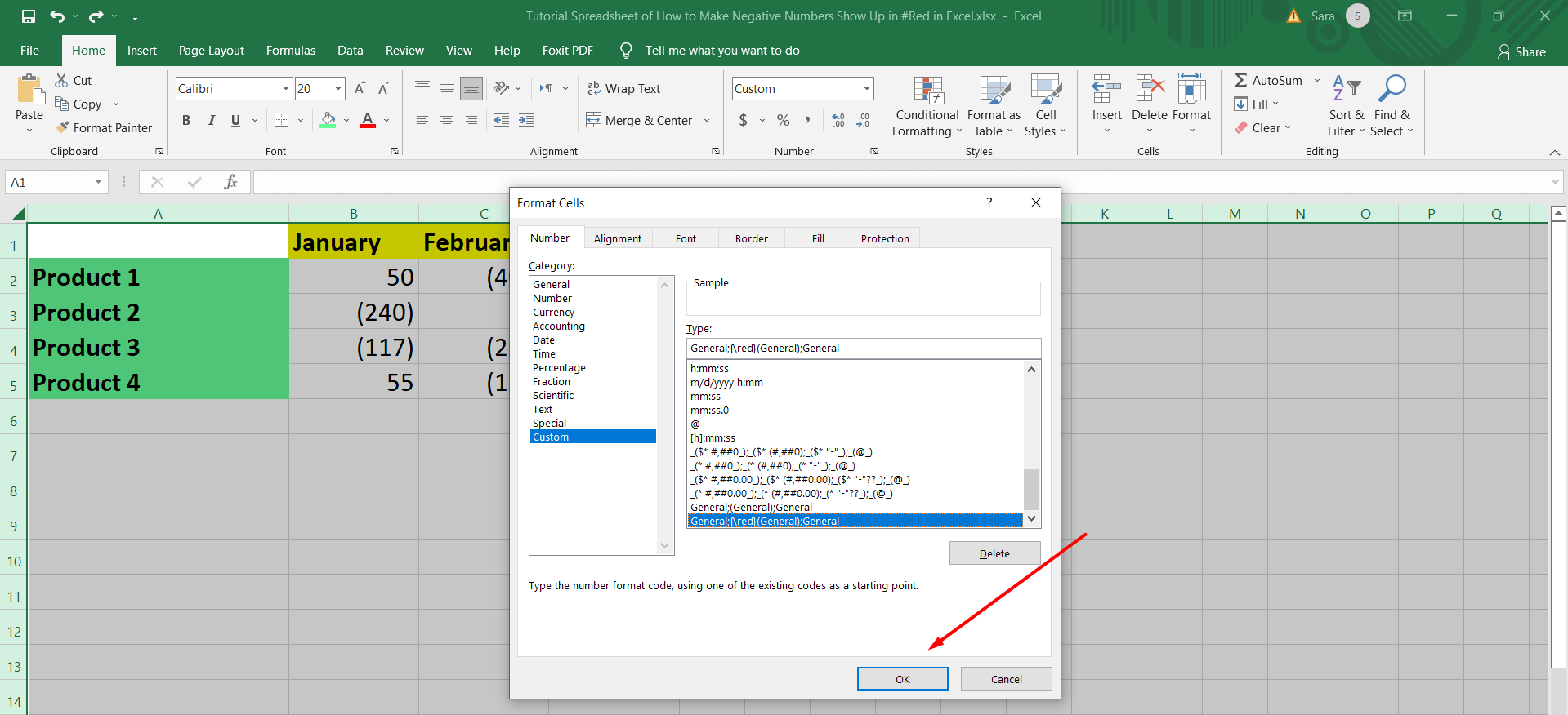Now, you can find the format cells of the whole numbers - the negative numbers- in red. That will show a significant difference in your work Excel spreadsheet format number.

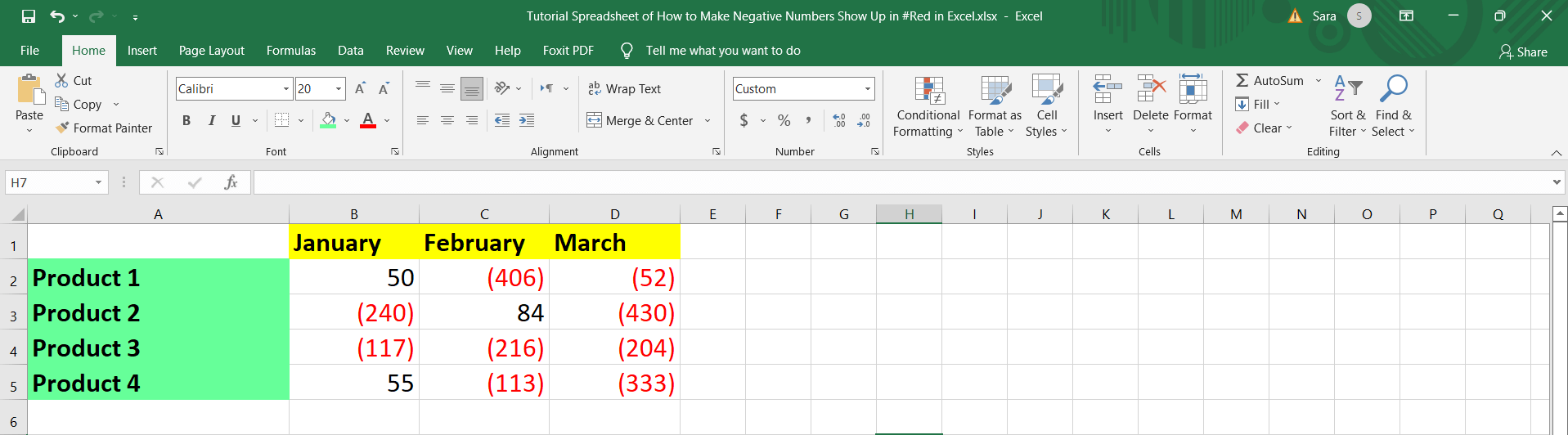
How Can I Add The Minus Sign To The Negative Numbers Cell-based

You can change the cell formatting to add the minus sign to the negative values cells. This formatting will not affect positive numbers. Step One: Please select all the cells in the workbook by highlighting them by clicking on the arrow on the top left side of the file. 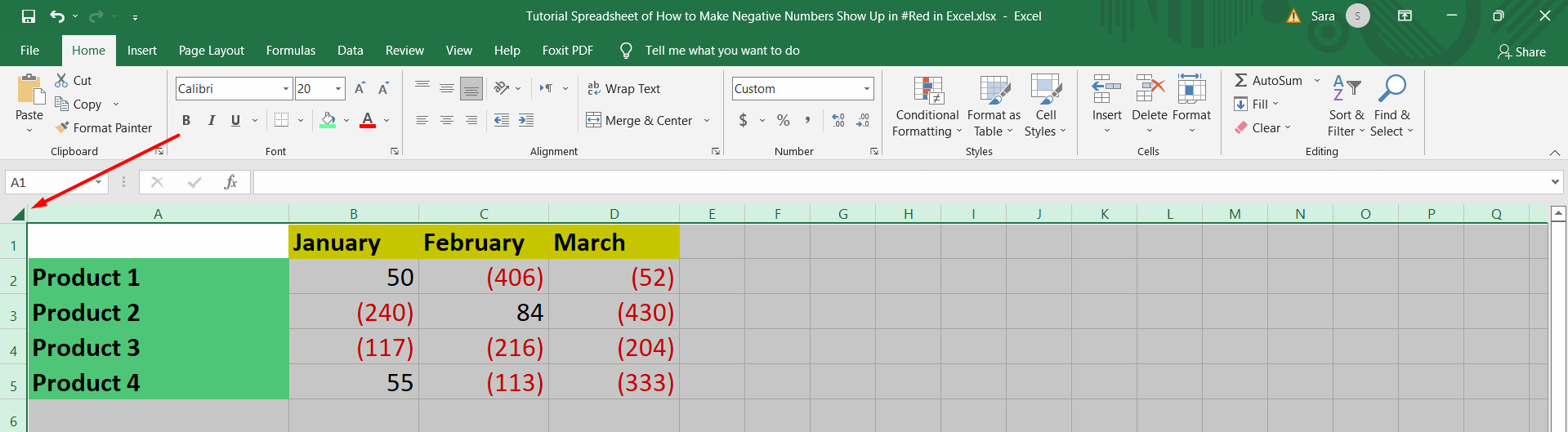Step Two: Click the right button on the mouse. Select the Format Cells dialog box option to custom formats. As shown below. Step Three: Choose "Custom Format," and then you can add the minus sign (-) beside the second "General" to create the formula making a negative number format in the Excel sheet. Or, copy the following formatting and paste it there: General;[red](-General); General 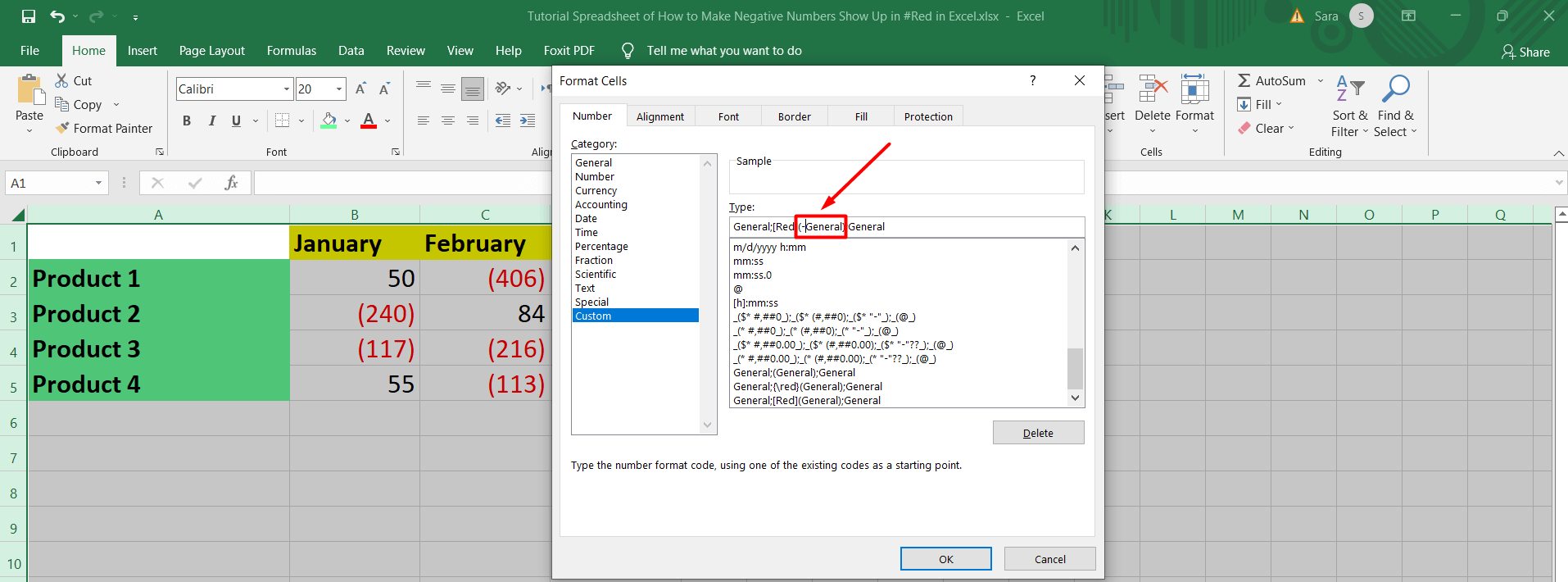Step Four: Click the OK button. 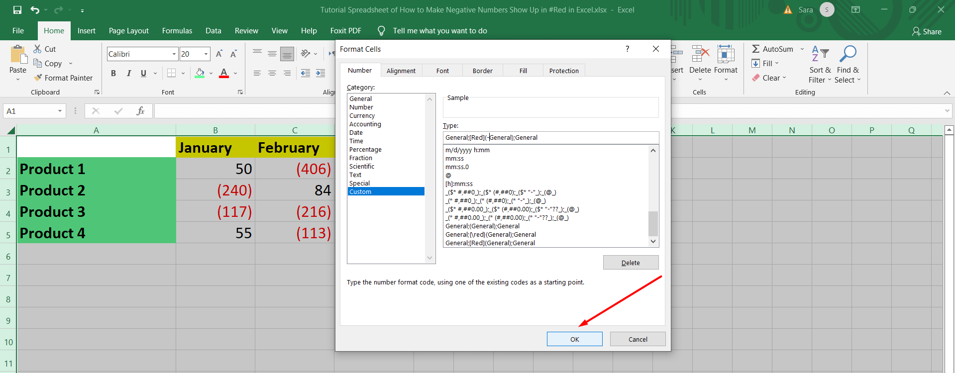Here, see the following screenshot of how the values formats will be.

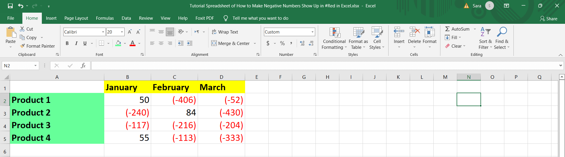
How Can I Change The Number Zero (0) To a (-) Sign

Step One: Highlight cells by clicking on the arrow on the top left side of the file. 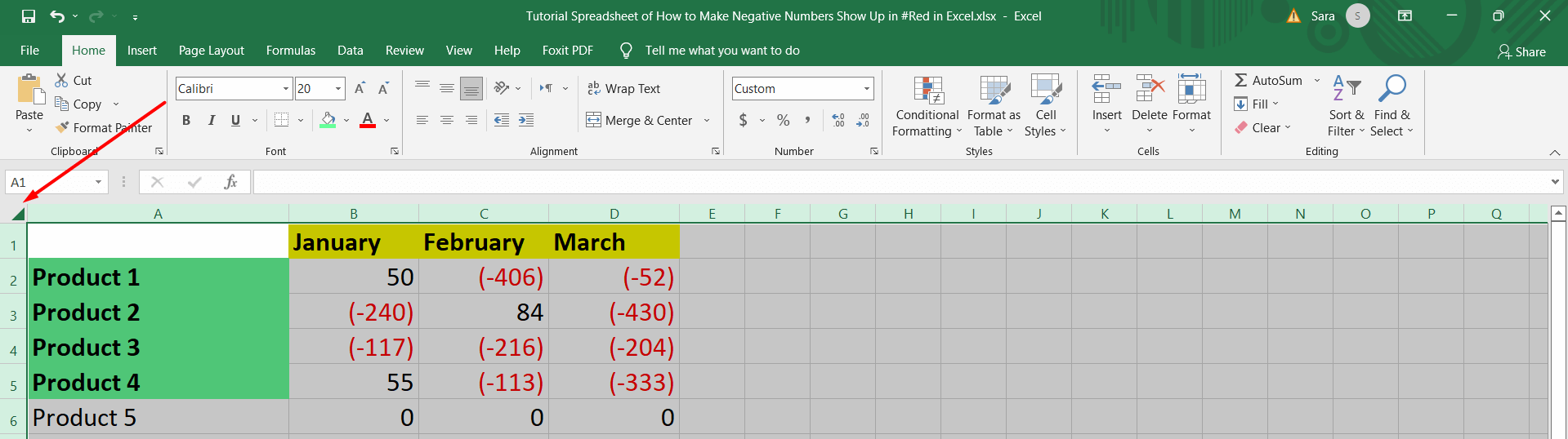Step Two: Click the right button on the mouse. Select the Format Cells option. 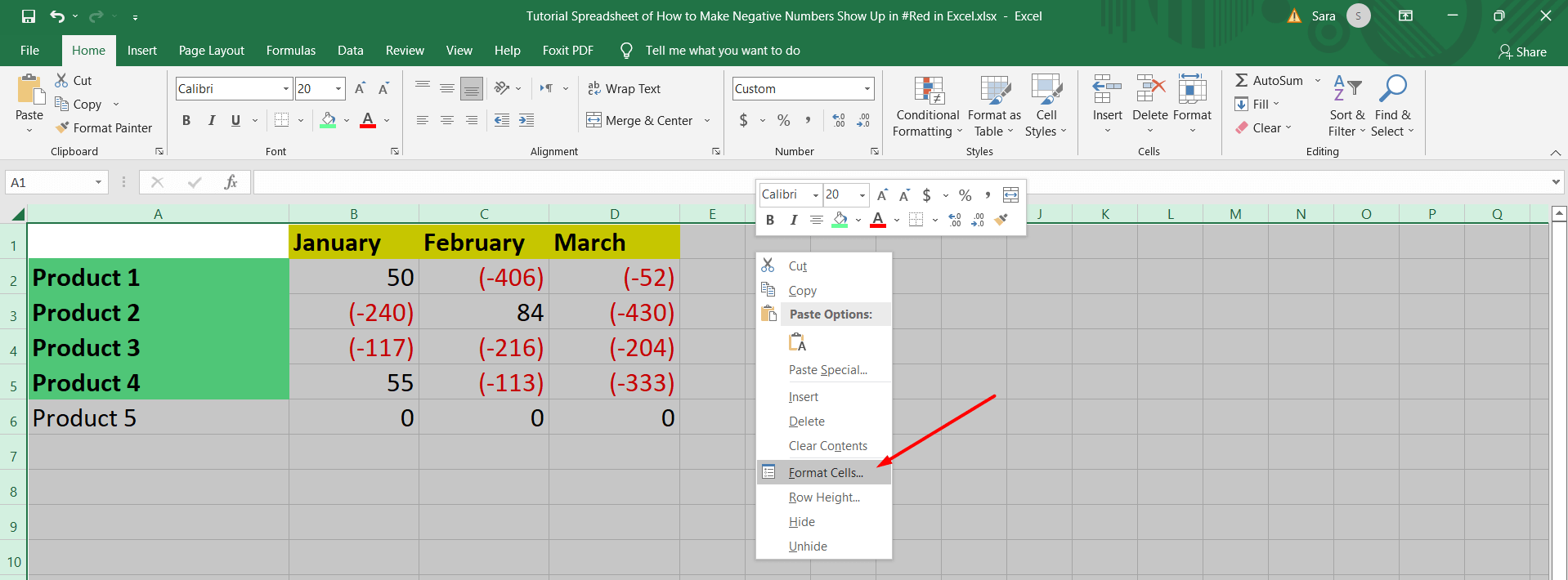Step Three: In the number tab, replace the third "general" with the sign (-) Or, copy the following formula General;[red](-General);- 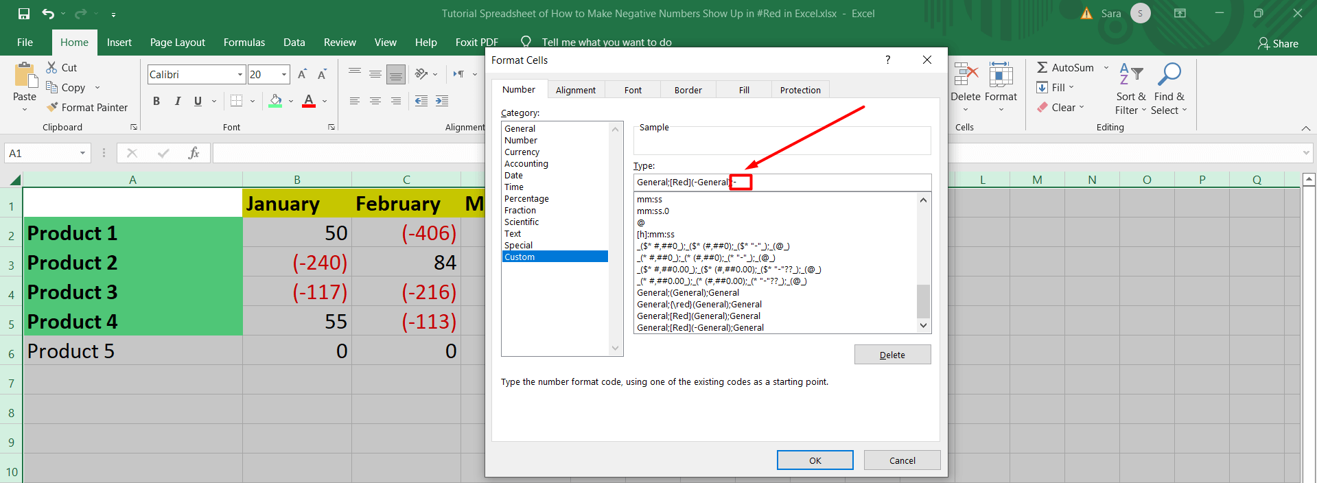Step Four: Save the formatting and click OK. 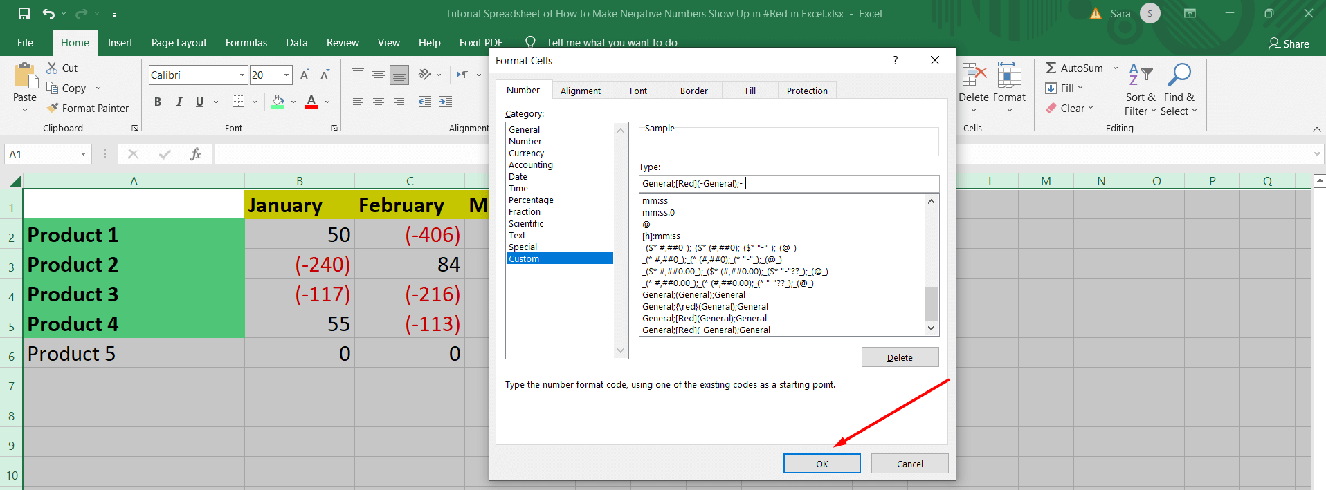Now, See the final negative number format after

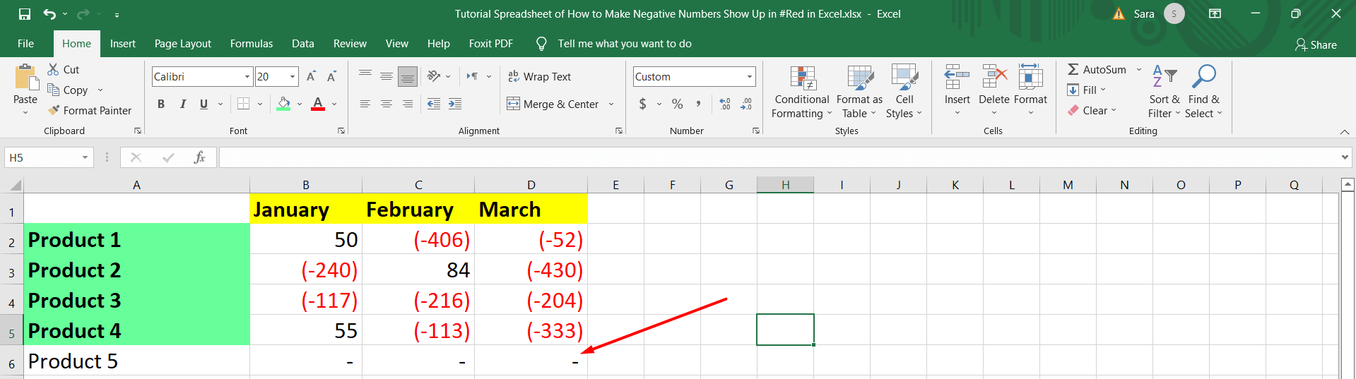
Note:

The Zero-value still appears in the original bar up the screen; it will only be changed in the cells. As shown below.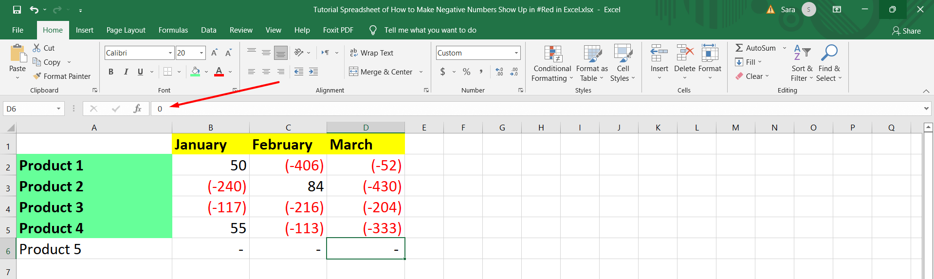

Using Conditional Formatting

The above method lets you understand how to create conditional formatting in your spreadsheets manually. If you want to achieve similar results in under two minutes, use the Conditional Formatting tool readily available in Excel. Head over your Ribbon in the Home Tab. In the Styles Group, click on Conditional Formatting. In the drop-down list, we can select Highlight Cells Rule > Less than, and enter 0 (since all values less than 0 are negative) And there you have it! Easy peasy! As mentioned in this post, excel makes your work life easier. You have to practice this feature while working on Excel. See our post, 10 Reasons Why Microsoft Excel is Fun. See the ready-to-use templates from the Simple Sheets website to facilitate the working range. See Excel Spreadsheet Templates: Microsoft Office (and the Field) vs. Simple Sheets. You can also use Printable Spreadsheet Templates to save time and resources.