
Excel Cannot Group Dates in Pivot Table: 3 Quick Fixes to Try.
Aug 25, 2022
The date grouping option in Microsoft Excel is a powerful tool that, if used correctly, can save you plenty of time and effort.
It allows you to analyze data in a large worksheet while grouping your data into dates, weeks, months, or years. Date grouping in pivots is exactly how an expense report with pivot consolidation summarizes monthly travel costs.
However, the gate grouping option doesn't always work. Sometimes, you will notice that the Group Field button from the Analyze tab of your pivot table ribbon is greyed out or disabled.
This article will examine why we cannot group dates in a pivot table and how to rectify this issue.
Suggested read: How to Connect Slicers to Multiple Pivot Tables
3 Methods to Solve Group Dates Problem in Pivot Table
Option 1: Replace Missing or Distorted Date Values with Group Dates in Pivot Table
Step 1:
The only way to get around this error while you use the Group Field tool for dates is to ensure all the cells from your date columns within the source data contain dates or blank cells.
If any cells within your data field include errors or text, the date grouping feature will not work, and the grouping feature will tell you that you cannot group that selection.
This is often due to issues in your pivot table's date field. To rectify these issues, you must insert dates into cells with no date value.
Step 2:
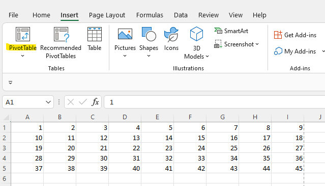
Next, let's group data together. To do this, we need to create a pivot table. Select the Insert tab, and choose the Pivot Table button from your Insert ribbon. Then, choose the data you want to implement and the location for your pivot table.
Step 3:
Once your pivot table is created, highlight some of the cells you want to group. Right-click on those chosen cells and a small window will show. Select Group from that window.
Another window will now appear, called Grouping. Here, you can choose how you want to group your data.
Once chosen, select OK.
If this hasn't worked, you will be shown an error message. Double check you have followed all of the steps highlighted above.

Suggested read: Excel Pivot Table Traning
Option 2: Filter to Find Out Distorted Date Values
Now let's focus on some ways to understand the error date values in your pivot table. There are three simple ways to gather these dates. The first is to use the filter to gather the date values that contain errors.
Step 1:
Choose every cell from the data range. Select the filter option from the Data tab.

Next, select the small downward arrow located next to Ship Date. You will notice the filter drop-down menu has grouped every date value. All text and error date values are at the bottom of the list.
Step 2:
You might notice that the column contains dates that have gotten entered in the incorrect format. Because of this, Excel does not deem these dates as dates when they were input in the cell and instead marks them as text.
To filter the Text and ERROR values, you need to uncheck all the date items, or you can remove the tick from the Select All option. After this, choose the text and error items.
Hit OK, and the column will not get filtered to only show the text values and error messages.
Step 3:
From there, it is time to understand why these values are getting deemed correct and amend them. Once this is complete, you can select the Filter option once more.
The data range will return to its initial state, with the correct dates now included.
Suggested Read: How To Fix a Reference Isn't Valid Error in Excel.
Option 3: Locate the Error Date Values Via the GoTo Special Menu to Group Dates in Pivot Table
Another option is the Go To Special menu, an excellent feature that lets you choose cells containing different data, including blanks, comments, formulas, constants, and more.
Steps:
Firstly, choose the entire column of the data field. To do this, press the CTRL+SPACE simultaneously.
Head to Find and Select from the Home tab, and choose to Go To Special.
Then choose the Constants button, and uncheck the Numbers button before hitting OK.
Any cells containing text or error values will get selected. Now apply a different fill color to highlight those cells, which will help you fix them in the next step.
Pivot Table Grouping: Summary and Key Takeaways
From this article, you know how to solve the pivot table grouping issue to ensure all the date values in your spreadsheet are accounted for. Working with two pivot tables or more can be extremely tricky, so getting these basics nailed first is essential before moving on to more advanced pivot table work. Pivot-grouped dates also feed neatly into a gantt chart timeline template when you need to visualize phases by month or quarter.
If you liked this article, check out the other content on the Simple Sheets blog or our YouTube channel.
Frequently Asked Questions About Pivot Table Grouping:
What is an Excel Pivot Table?
A pivot table is the best interactive way to analyze and summarize large quantities of data. Pivot tables are perfect for analyzing numerical data and are ideal for large amounts of data.
Can you create Excel pivot tables in blank cells?
You can place your pivot table on a blank cell, but you will need to link it to data in your spreadsheet, or no data will show in the pivot table.
How do standard pivot tables work?
A pivot table is a perfect tool for showing large quantities of data. Once you have set up your pivot tables based on your data, you can start dragging and dropping sections to show data in a way that suits your needs.
Related Articles:
Excel: Remove Trailing Spaces Quickly and Easily With These Simple Steps
Want to Make Excel Work for You? Try out 5 Amazing Excel Templates & 5 Unique Lessons
We hate SPAM. We will never sell your information, for any reason.

