Learn Different Ways to Use the IFS and VLOOKUP Nested Function
Jul 15, 2023
Do you want an Excel formula that can save time and simplify worksheet management?
Quick answer: Nesting means putting a VLOOKUP inside an IF or IFS so the lookup result becomes the thing being tested. For two outcomes use =IF(VLOOKUP(H4,$B$4:$E$12,4,FALSE)=0,"No","Yes"). For three or more, swap IF for IFS and finish with TRUE as the catch-all condition.
Last updated: August 24, 2026
Get our free Excel formulas cheat sheet
Plus new tutorials and template drops. Enter your email and we'll send it over.
Combining these two functions lets you use the strengths of both. VLOOKUP finds the number, IF or IFS decides what to do about it, and you stop retyping information by hand.
People search for this in a dozen ways: nested VLOOKUP, VLOOKUP IFS, IFS with VLOOKUP, IF and VLOOKUP together, nested IF VLOOKUP, VLOOKUP if statement, VLOOKUP if else, or simply how to combine VLOOKUP and IF. They all mean the same thing, and every formula below is written out in full so you can copy it.
You will also see it written up as IFS VLOOKUP, VLOOKUP with IFS, nested IF with VLOOKUP, IF then VLOOKUP, or VLOOKUP with IF condition. If you came here looking for how to use IF and VLOOKUP together, or for VLOOKUP with AND function, both patterns are covered further down.
Read on as we cover the following:

How nesting IF and VLOOKUP actually works
Nesting means one function sits inside another as an argument. The inner one runs first and hands its answer up.
You can use the IF statement to set a condition, and VLOOKUP is a reference function that looks for a particular value within a range. Put the VLOOKUP inside the IF and the lookup result becomes the thing being tested.
Rule: The VLOOKUP goes in the first argument of IF, the logical test. It does not go in the second or third argument unless you want the lookup to be the answer rather than the question.
All the examples on this page use one dataset. Products run down rows 4 to 12, with column B holding the product ID, column C the product name, column D the unit price and column E the quantity in stock. The product ID you are searching for is typed into cell H4. Swap the ranges for your own and the shape of every formula stays the same.
Because the lookup range is written as $B$4:$E$12 with dollar signs, you can fill any of these formulas down a column without the range sliding out from under it.
IF or IFS? Which one you should nest
This is the fork that decides everything else, and it is the reason so many of these formulas come out as a wall of brackets.
| IF | IFS | |
|---|---|---|
| Shape | =IF(test, value_if_true, value_if_false) | =IFS(test1, value1, test2, value2, ...) |
| Outcomes | Exactly two | As many as you like |
| Three or more bands | You must nest IF inside IF inside IF | Just keep adding pairs, no nesting |
| The else branch | Built in, the last argument | None. Finish with TRUE as the final test |
| If nothing matches | Returns the false value | Returns #N/A |
| Available in | Every version of Excel | Excel 2019, 2021, Microsoft 365, Excel for the web |
Rule: IFS does not exist in Excel 2016 perpetual, 2013 or 2010. Typing it there returns #NAME?. If your file has to open on an older machine, use nested IF instead and everything else on this page still works.
1. Use IF and VLOOKUP to match a specific value
The classic job: look up a product and report whether it is in stock. Two outcomes, so IF is the right choice.
=IF(VLOOKUP(H4,$B$4:$E$12,4,FALSE)=0,"No","Yes")
In our example, the dataset includes the products' ID, name, unit price and quantity in stock.
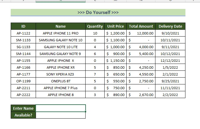
Checking stock availability this way is the same lookup pattern that drives an inventory excel template. Follow the steps below.
-
Select the cell where you want the answer.
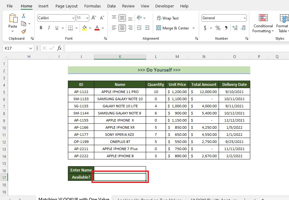
-
Type =IF( and then start the VLOOKUP inside it as the logical test.
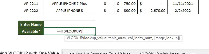
-
Finish the VLOOKUP, compare it to 0, then add the two outcomes and close both brackets.
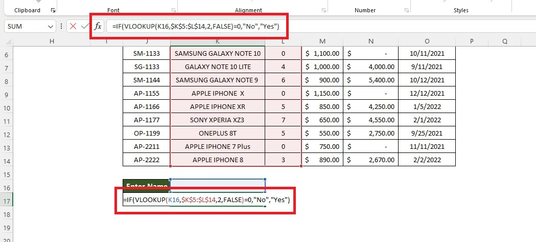
-
Press Enter, then type a product ID into H4 to trigger it.
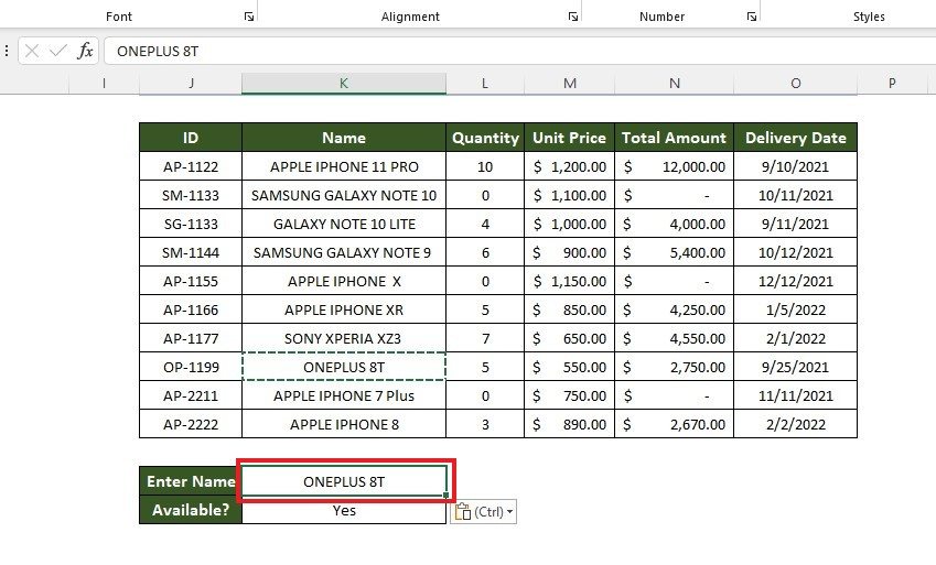
Formula breakdown:
-
H4 is the cell holding the product ID you are searching for.
-
$B$4:$E$12 is the range being searched. VLOOKUP always matches against the first column of that range, which is column B, the product ID.
-
4 counts four columns across from B, landing on column E, the quantity in stock. Count the columns in your own range rather than guessing, because getting this number wrong returns the right-looking answer from the wrong column.
-
FALSE forces an exact match. Leave it out and Excel assumes an approximate match, which needs the first column sorted and silently returns nonsense when it is not.

So VLOOKUP returns the quantity, and the IF function returns Yes or No depending on whether that quantity is zero.

Rule: Read the arguments in order. IF asks the question, the second argument is what happens when the answer is yes, the third is what happens when it is no. Swapping those two is the most common way a nested formula ends up backwards while still calculating without an error.
2. Use IFS and VLOOKUP to sort results into three or more bands
IF gives you two outcomes. The moment you need three, nested IF turns into brackets inside brackets. IFS was built for exactly this.
Say you want to label each product Premium, Standard or Budget based on its unit price:
=IFS(VLOOKUP(H4,$B$4:$E$12,3,FALSE)>=800,"Premium",VLOOKUP(H4,$B$4:$E$12,3,FALSE)>=300,"Standard",TRUE,"Budget")
IFS reads as a list of pairs: test, answer, test, answer. It works down the list and stops at the first test that comes back TRUE. Column 3 of the range is column D, the unit price.
The final pair, TRUE,"Budget", is the catch-all. TRUE is always true, so anything that fell through the earlier tests lands there. Leave it off and a product under 300 returns #N/A, because IFS has no built-in else branch.
The same logic written with nested IF, for anyone on an older build:
=IF(VLOOKUP(H4,$B$4:$E$12,3,FALSE)>=800,"Premium",IF(VLOOKUP(H4,$B$4:$E$12,3,FALSE)>=300,"Standard","Budget"))
Rule: Order your IFS conditions from most restrictive to least. Put the 300 test before the 800 test and every premium product gets labelled Standard, because IFS stops at the first match and never looks further down the list.
3. Look up based on two values
Each product in this dataset has two market prices, in columns D and E. You want to say which product and which market, then get the right price back.
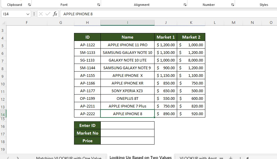
Type the product ID into H4 and the market number, 1 or 2, into I4.
=IF(I4=1,VLOOKUP(H4,$B$4:$E$12,3,FALSE),VLOOKUP(H4,$B$4:$E$12,4,FALSE))
-
Enter the formula in the result cell.
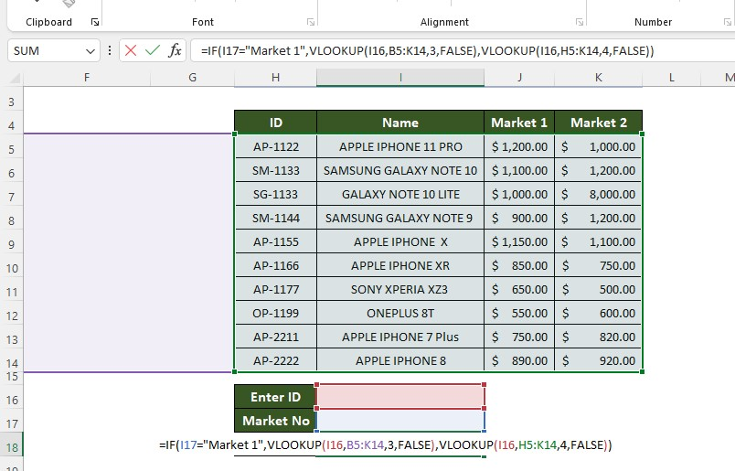
-
Type the ID and the market number to trigger it.
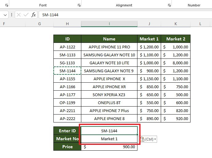
Formula breakdown: I4=1 is the logical test. If the market number is 1, the first VLOOKUP runs and pulls from column 3. Otherwise the second VLOOKUP runs and pulls from column 4. This is also a neat answer to looking up based on multiple values without an array formula.

Rule: Test a number against a number. I4=1 works when the cell holds the number 1. I4="Market 1" works when it holds that text. Mixing the two, testing I4="Market 1" while the reader types 1, never errors. It just quietly returns the wrong branch every single time.

Once you have three or more markets, swap IF for IFS rather than nesting:
=IFS(I4=1,VLOOKUP(H4,$B$4:$F$12,3,FALSE),I4=2,VLOOKUP(H4,$B$4:$F$12,4,FALSE),I4=3,VLOOKUP(H4,$B$4:$F$12,5,FALSE))
Or skip the branching entirely. Because market 1 lives in column 3, market 2 in column 4 and so on, the market number plus two is the column index:
=VLOOKUP(H4,$B$4:$F$12,I4+2,FALSE)
Conditional pricing logic like this is exactly the pattern behind a simple purchase order template, where unit cost depends on vendor or quantity break.
4. Match a lookup return against another cell
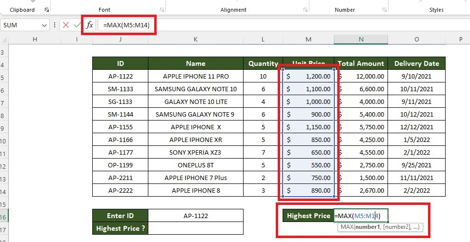
Here we use the MAX function to find the highest price in the data, then compare the looked-up price against it.
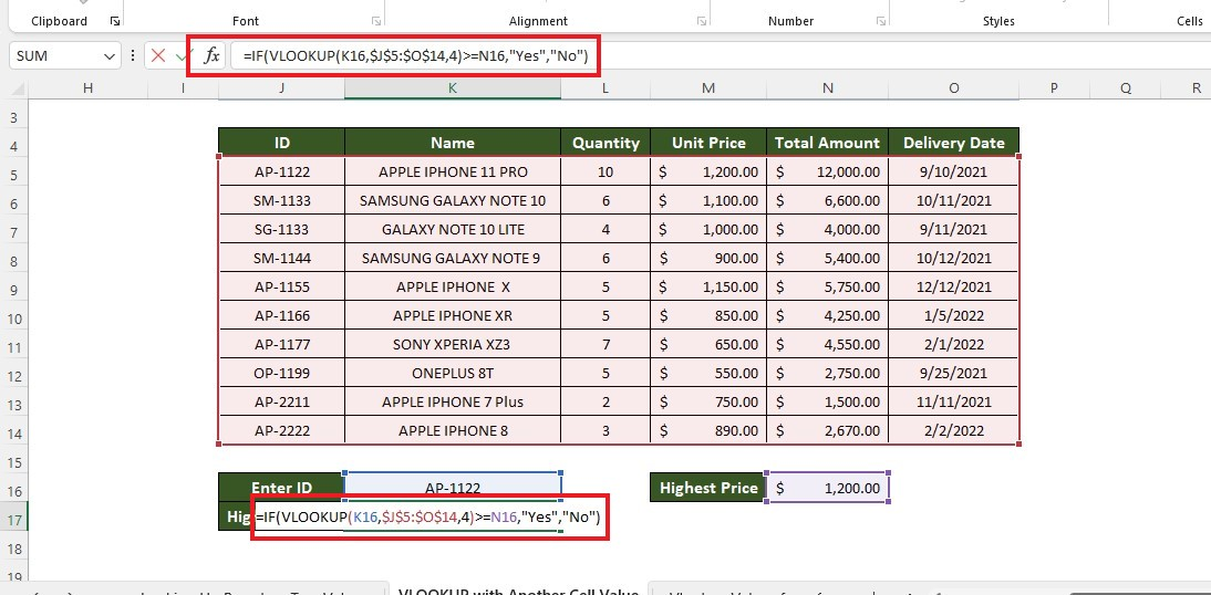
=IF(VLOOKUP(H4,$B$4:$E$12,3,FALSE)>=MAX($D$4:$D$12),"Yes","No")
-
Work out the highest price first with =MAX($D$4:$D$12), so you can see the number you are comparing against.
-
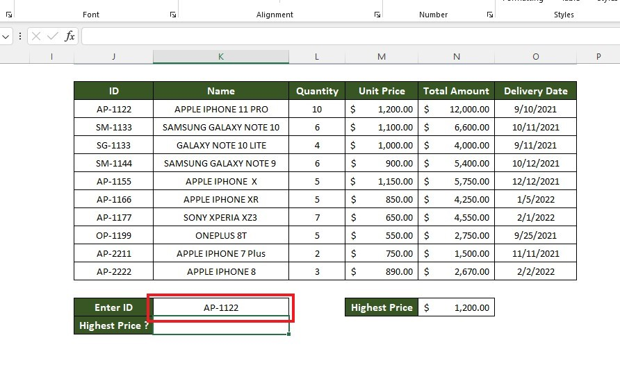
Type the product ID you want to test into H4.
-
Build the IF around the VLOOKUP, comparing it to MAX.
-
Press Enter to get the result.
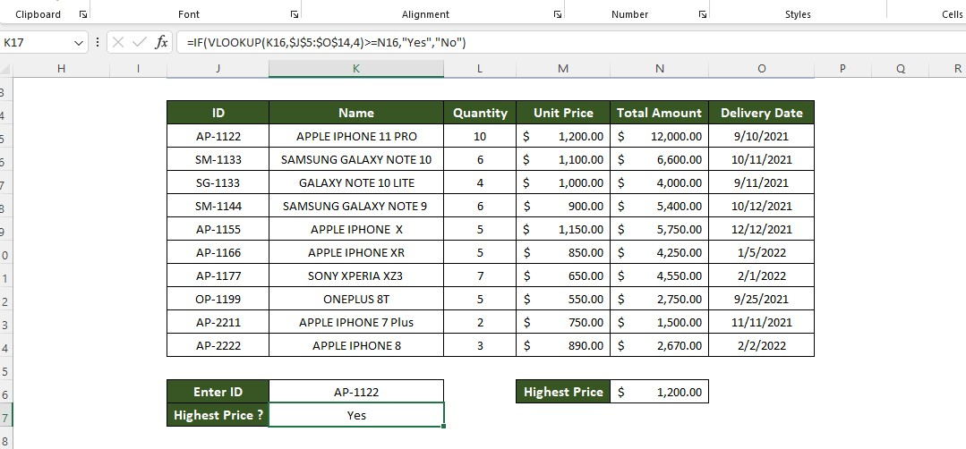
Formula breakdown: the VLOOKUP returns the price for the ID in H4. MAX returns the highest price anywhere in column D. If the first is greater than or equal to the second, the formula prints Yes, otherwise No.

5. Look up values from a shorter list with ISNA
A common job: you have a full product list and a much shorter "Delivered" list, and you want to mark each product Delivered or Not Delivered. VLOOKUP alone returns #N/A for everything missing from the short list, which is ugly and unusable. Wrapping it in ISNA turns that error into a useful label.
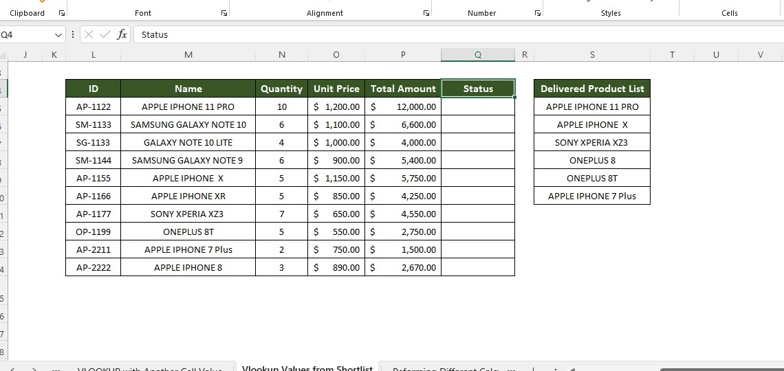
=IF(ISNA(VLOOKUP(B4,$H$4:$H$8,1,FALSE)),"Not Delivered","Delivered")
-
Select the first cell under the Status column.
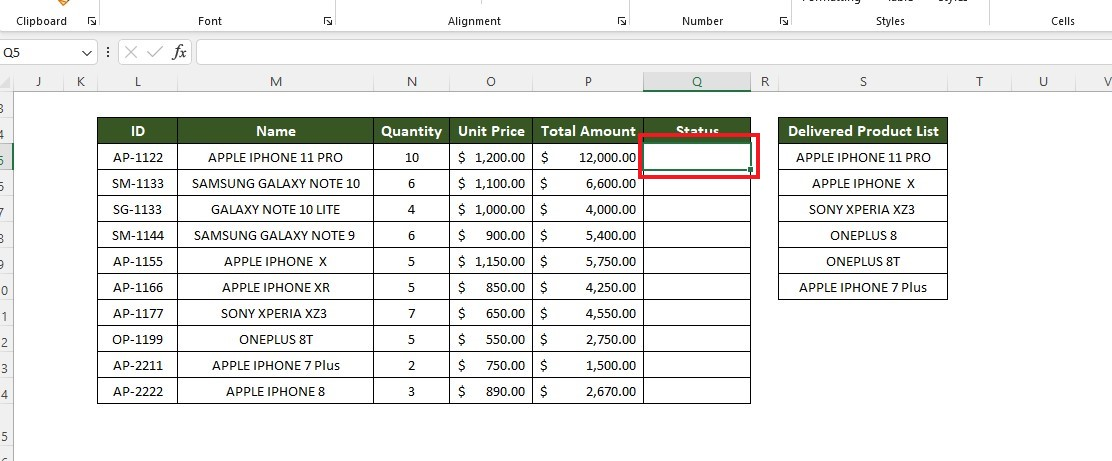
-
Type the formula and press Enter.
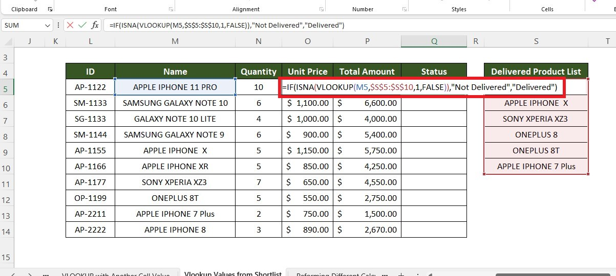
-
Use the fill handle to fill the other rows.
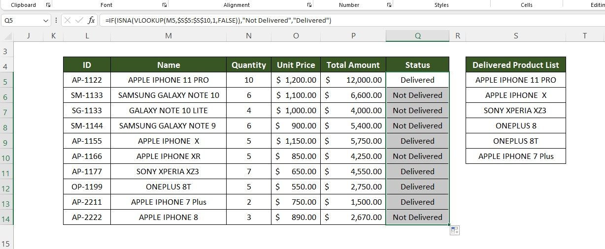
Formula breakdown: ISNA asks one question, is this thing #N/A, and returns a Boolean value, TRUE or FALSE. A missing product makes VLOOKUP throw #N/A, ISNA turns that into TRUE, and IF prints "Not Delivered". A product that is found makes ISNA return FALSE, so IF prints "Delivered".
Rule: This is the one formula on the page you are told to fill down, so the lookup range must be locked with dollar signs. Written as H4:H8 instead of $H$4:$H$8, the range slides down one row per row as you fill, and products near the bottom get marked Not Delivered when they were delivered. Nothing errors. The column just quietly fills with wrong answers.
6. Perform different calculations from one lookup
Nesting is not only for text labels. The two branches of an IF can each be a calculation.
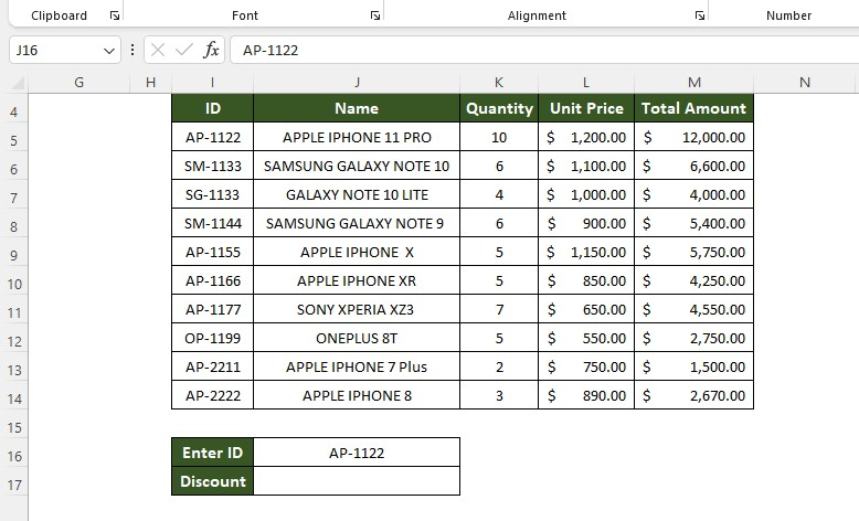
The rule we are building: products priced above 800 get a 20% discount. Products at 800 or below get 15%.
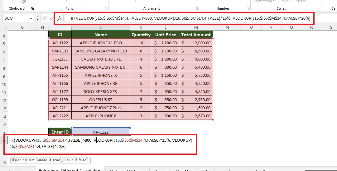
=IF(VLOOKUP(H4,$B$4:$E$12,3,FALSE)>800,VLOOKUP(H4,$B$4:$E$12,3,FALSE)*0.2,VLOOKUP(H4,$B$4:$E$12,3,FALSE)*0.15)
-
Type the product ID into H4.
-
Type the formula into the result cell.
-
Press Enter to get the discount amount.
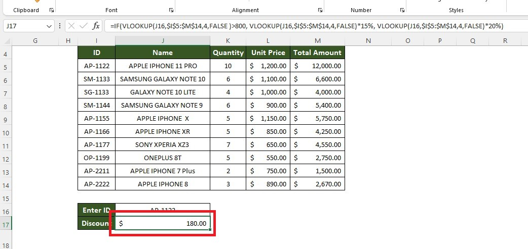
Formula breakdown: the first VLOOKUP checks whether the unit price for the ID in H4 is above 800. If it is, the second VLOOKUP runs and multiplies that same price by 0.2, giving a 20% discount. If it is not, the third VLOOKUP multiplies by 0.15 for 15%.

To return the price the customer actually pays rather than the discount, multiply by 0.8 and 0.85 instead of 0.2 and 0.15.

Rule: Write the discount rule down in plain words before you write the formula, then read the finished formula back against it. A 20% discount is a multiplier of 0.2 if you want the discount and 0.8 if you want the price. Getting those two backwards produces a perfectly valid formula that is wrong on every row.
7. Test two conditions at once with AND
Sometimes one condition is not enough. Nest AND inside the IF to require both.
=IF(AND(VLOOKUP(H4,$B$4:$E$12,3,FALSE)>500,VLOOKUP(H4,$B$4:$E$12,4,FALSE)>0),"Order now","Hold")
This reads: if the price is above 500 and there is stock left, say Order now, otherwise say Hold. Swap AND for OR when either condition is enough on its own. Using VLOOKUP with the AND function this way is far easier to read than three nested IFs.
8. Stop the #N/A errors with IFNA
The ISNA method in section 5 is the classic. There is a shorter modern version.
| Formula | Catches | Works in |
|---|---|---|
| =IFNA(VLOOKUP(H4,$B$4:$E$12,2,FALSE),"Not found") | Only #N/A, so real errors still surface | Excel 2013 and later |
| =IFERROR(VLOOKUP(H4,$B$4:$E$12,2,FALSE),"Not found") | Every error, including your own mistakes | Excel 2007 and later |
| =IF(ISNA(VLOOKUP(H4,$B$4:$E$12,2,FALSE)),"Not found",VLOOKUP(H4,$B$4:$E$12,2,FALSE)) | Only #N/A | Every version |
IFNA is the one to reach for. IFERROR is tempting because it catches everything, and that is exactly the problem: it hides a #REF! from a deleted column just as cheerfully as it hides a genuine not-found, so a broken formula looks fine for months.
Troubleshooting
| What you see | Why | Fix |
|---|---|---|
| #N/A | The lookup value is not in the first column of the range, or it is misspelled, or it has a trailing space, or one side is a number stored as text | Check the spelling, wrap the lookup value in TRIM, and wrap the whole thing in IFNA |
| #NAME? | IFS or IFNA does not exist in your version of Excel, or the function name is mistyped | Use nested IF instead of IFS, and the ISNA version instead of IFNA |
| #N/A from IFS specifically | None of the conditions came back TRUE and IFS has no else branch | Add TRUE as the final condition, paired with your catch-all answer |
| #REF! | col_index_num is bigger than the number of columns in the range | Count the columns in the range again. $B$4:$E$12 is four columns wide, so 5 is out of bounds |
| #VALUE! | col_index_num is less than 1, or a text value ended up in a calculation branch | The column index must be 1 or higher, and both branches of an arithmetic IF must return numbers |
| The answer is the opposite of what it should be | The value_if_true and value_if_false arguments are the wrong way round | Read the formula out loud as a sentence. Second argument means yes, third means no |
| It works on row 4 but goes wrong further down after filling | The lookup range is relative and slides with each row | Lock it with dollar signs, $B$4:$E$12, or convert the source data to an Excel Table |
| Everything lands in one band with IFS | The conditions are ordered from least restrictive to most, so the first one catches everything | Reorder from most restrictive down |
| Too many brackets to follow | Three or more nested IFs | Rewrite it as a single IFS, or split the lookup into a helper column and test that |
Final thoughts on the IFS and VLOOKUP nested function
Nesting IFS or IF around a VLOOKUP lets you pull a number out of a table and act on it in the same cell. Drawing on multiple conditions turns a lookup into a decision with very little user input.
Nested lookups like this also show up in BOM costing, where a bill of materials spreadsheet rolls component prices into an assembly total.
Visit Simple Sheets for more easy-to-follow Excel guides and financial model examples, and remember to visit the related articles section of this blog post.
For the most straightforward Excel video tutorials, subscribe to Simple Sheets on YouTube!
Frequently asked questions on the IFS and VLOOKUP nested function
How do you nest IFS and VLOOKUP in Excel?
Put the VLOOKUP inside IFS as a logical test, so the lookup result is the thing being judged. For example =IFS(VLOOKUP(H4,$B$4:$E$12,3,FALSE)>=800,"Premium",VLOOKUP(H4,$B$4:$E$12,3,FALSE)>=300,"Standard",TRUE,"Budget"). The final TRUE pair is the catch-all, because IFS has no built-in else branch.
What is the difference between IF and IFS with VLOOKUP?
IF handles exactly two outcomes and has a built-in else. IFS handles any number of outcomes as test and answer pairs, but has no else, so you finish with TRUE. Use IF for yes or no questions and IFS the moment you need three or more bands, rather than nesting IF inside IF.
What is the IF and VLOOKUP formula in Excel?
The standard shape is =IF(VLOOKUP(lookup_value, range, column_number, FALSE)=test_value, "answer if true", "answer if false"). A working example is =IF(VLOOKUP(H4,$B$4:$E$12,4,FALSE)=0,"No","Yes"), which reports whether a product is in stock.
How many IF statements can I use?
Excel allows up to seven levels of nesting in versions 2003 and older. For versions 2007 and newer you can nest up to 64 IF functions in a single formula. Long before you reach either limit the formula becomes unreadable, so switch to IFS or a helper column at around three.
Why do I get an #N/A error with VLOOKUP?
The usual causes are a misspelled lookup value, a lookup value that is genuinely missing from the first column of the range, a range that does not start at the column you are matching against, or a number on one side and text on the other. Trailing spaces are the sneakiest of these.
Is there a function to avoid #N/A errors using IF and VLOOKUP?
Yes. Use =IFNA(VLOOKUP(H4,$B$4:$E$12,2,FALSE),"Not found") on Excel 2013 or later. On older versions, the ISNA combination does the same job: =IF(ISNA(VLOOKUP(H4,$B$4:$E$12,2,FALSE)),"Not found",VLOOKUP(H4,$B$4:$E$12,2,FALSE)).
Can I use VLOOKUP with two conditions in an IF statement?
Yes. Nest AND inside the IF: =IF(AND(VLOOKUP(H4,$B$4:$E$12,3,FALSE)>500,VLOOKUP(H4,$B$4:$E$12,4,FALSE)>0),"Order now","Hold"). Swap AND for OR when either condition on its own is enough.
Why does my nested VLOOKUP break when I fill it down?
The lookup range is relative, so it slides down one row for every row you fill. Lock it with dollar signs, for example $B$4:$E$12, or convert the source data to an Excel Table and use the table name. Nothing errors when this happens, the answers just go quietly wrong.
Related Articles
What is a Sunburst Chart and When to Use a Sunburst Chart in Excel
Want to Make Excel Work for You? Try out 5 Amazing Excel Templates & 5 Unique Lessons
We hate SPAM. We will never sell your information, for any reason.