
The Beginners Guide on Reverse VLOOKUP in Excel
Jul 05, 2023
Have you ever had to reverse-lookup a value in Excel?
Figuring out how to search backward to return the right result can sometimes be tough.
Get our free Excel formulas cheat sheet
Plus new tutorials and template drops. Enter your email and we'll send it over.
Well, don't worry! In this blog post, we'll discuss some simple and versatile techniques for performing a reverse VLOOKUP in Excel.
Whether you're trying to look up numbers or words, these methods will save you time and effort while helping ensure accuracy every time.
Read on as we cover the following:
-
Reverse VLOOKUP in Excel
-
INDEX and MATCH Functions for Reverse Lookup
-
Final Thoughts on Reverse VLOOKUP in Excel
-
Frequently Asked Questions on Reverse VLOOKUP in Excel

Reverse VLOOKUP in Excel
To reverse the Excel VLOOKUP function, we must retrieve the original lookup values using the VLOOKUP and CHOOSE functions.
The VLOOKUP function syntax
The VLOOKUP function syntax:

The Excel VLOOKUP function requires the following arguments:
-
Lookup_value: the cell value we must find in the first column in the table.
-
Table_array: from which you can take out a lookup array.
-
Column_index_num: the column number from which we will return a value.
-
Range_lookup: the optional argument. Usually, it means approximate match, which is the default setting. If you want an exact match, change it to FALSE.
The VLOOKUP function searches for data in a vertically-organized table. It can match approximate and exact values and use wildcard characters (*, $) for partial matches.
The CHOOSE function syntax
The CHOOSE function syntax:

The Excel CHOOSE function requires the following arguments:
-
Index_num: The value to select a number between 1 and 254.
-
Value 1: First selected value
-
Value 2: The optional argument is the second value we must choose.
How to use the reverse VLOOKUP function
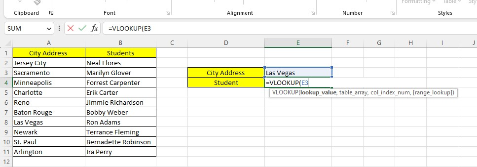
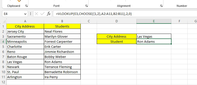
In our example, we'll find the student's name living in Las Vegas.
We should search for the city address in the "city address" lookup column and the corresponding student's name in the "students" column.
-
Type the VLOOKUP function and the lookup value.
-
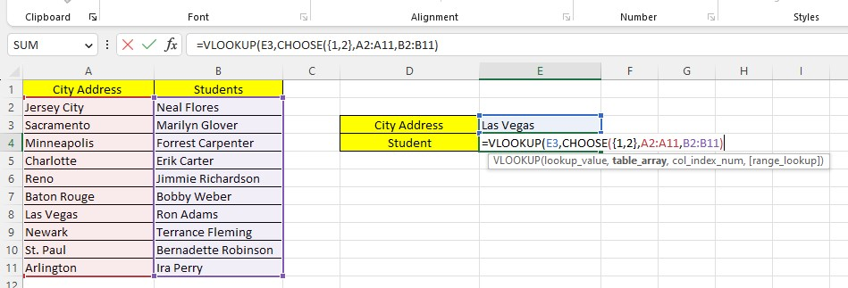
Type the index number, values 1 and 2 of the CHOOSE function.
-
Type the array constant.
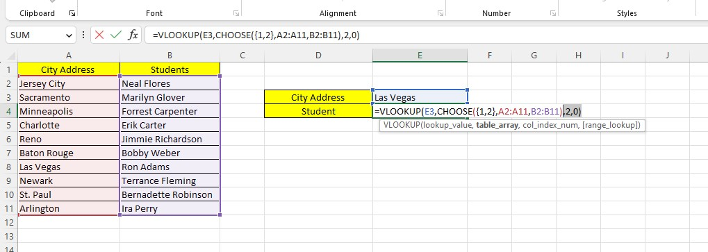
After pressing the Enter key, you now have the results of the reverse VLOOKUP formula.
INDEX and MATCH Functions for Reverse Lookup
To understand the use of the INDEX and MATCH functions as a reverse lookup formula:
-
The MATCH function shows a value's index location or cell number in a lookup column or row.
-
The INDEX function retrieves the lookup value of the cell number.
The INDEX function syntax
To learn more about the INDEX function, below is the syntax of the INDEX function:

The row_num argument of the INDEX function retrieves the row number. For example, if you type 5, the row_num will return the 5th-row value in your spreadsheet.
To have a reverse lookup formula, replace the MATCH function with the INDEX function row_argument.
How to use INDEX and MATCH functions for reverse lookup
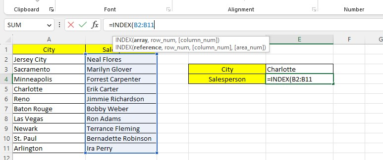
In our next example, we'll find the name of the salesperson working in Charlotte.
So, we'll search for the city from the "city" lookup column and the corresponding salesperson's name from the "salesperson" column.
-
Type the lookup column or the second column for the INDEX function.
-
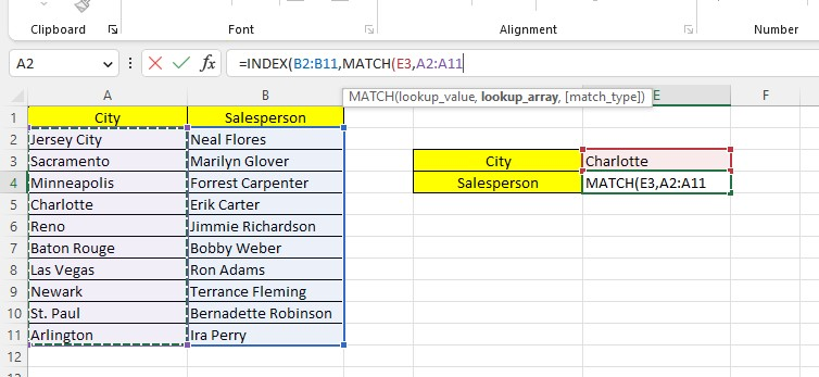
Type the MATCH function with its lookup cell and leftmost column value.
-
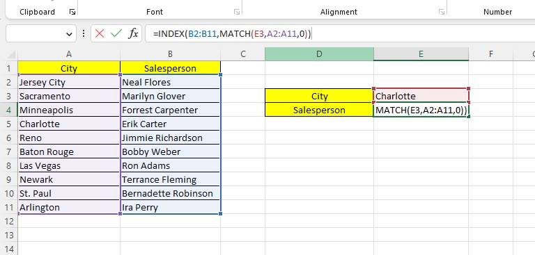
Type the exact match type and close the formula.
-
Press the Enter key.
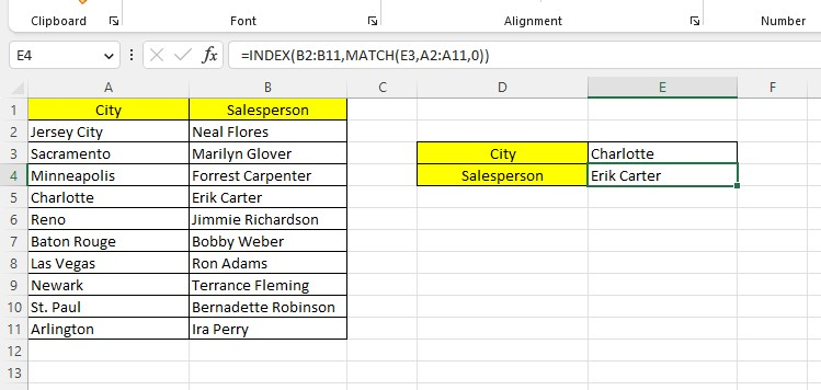
The formula returns the corresponding value according to the matching value of the city.
Final Thoughts on Reverse VLOOKUP in Excel
Reverse lookup in Excel is invaluable because it makes it much easier to cross-reference data between multiple sources.
The ease and speed of locating information using reverse lookups can be a game changer for anyone who wants to streamline their operations. Inventory work often needs reverse lookups — say finding a SKU from a partial description — so try our inventory spreadsheet template for a ready-made setup.
Visit Simple Sheets for more easy-to-follow Excel guides, and remember to read the related articles section of this blog post.
For the most straightforward Excel video tutorials, subscribe to Simple Sheets on YouTube!
Frequently Asked Questions on Reverse VLOOKUP in Excel
Are there any limitations or considerations when using reverse lookup in Excel?
The lookup column should contain unique values for accurate results. If there are duplicates, the lookup functions may return the first matching value, not necessarily the desired one.
Can I perform a reverse lookup with multiple criteria in Excel?
Yes, you can perform a reverse lookup with multiple criteria in Excel. To perform this, use the INDEX and MATCH functions and multiple conditions using the "&" operator.
How can the reverse lookup is different from the regular lookup?
Reverse lookup in Excel is finding a value in one column based on a corresponding value in another.
Related Articles
Beginners Guide: How To Group Dates In Pivot Table
CHOOSECOLS Function In Excel : The Only Guide You Need
Want to Make Excel Work for You? Try out 5 Amazing Excel Templates & 5 Unique Lessons
We hate SPAM. We will never sell your information, for any reason.

