How to Sum a Column in Google Sheets
Feb 14, 2023
Quick answer
To sum a column in Google Sheets, click an empty cell below your data, type =SUM(, drag over the numbers you want to add, then press Enter. To include every future row automatically, use an open range like =SUM(B2:B) and put the formula in a different column.
Last updated: August 20, 2026
Get our free Excel formulas cheat sheet
Plus new tutorials and template drops. Enter your email and we'll send it over.
Table of Contents
- Which method should you use?
- What is the formula to sum a column in Google Sheets?
- How do you sum a column with the SUM function, step by step?
- How do you sum an entire column that keeps growing?
- How do you use AutoSum in Google Sheets?
- How do you see a column total without typing a formula?
- How do you sum only the rows that match a condition?
- How do you sum only the visible rows after filtering?
- How do you sum the same column across several tabs?
- How do you build a running total down a column?
- Why is your sum returning 0 or the wrong number?
- What if you are working in Excel instead?
- Frequently asked questions
Which method should you use?
Six approaches cover almost every real spreadsheet. Pick by what your data is doing, not by which formula you saw first.
| Method | Use it when | Example |
|---|---|---|
| SUM, fixed range | The data has a known first and last row. | =SUM(B2:B25) |
| SUM, open range | Rows get added at the bottom over time. | =SUM(B2:B) |
| Status bar | You want a number to read, not a formula to keep. | Select the range, read the bottom right |
| SUMIF and SUMIFS | Only some rows should count, based on another column. | =SUMIF(C2:C, "Paid", B2:B) |
| SUBTOTAL | A filter is on and the total must follow it. | =SUBTOTAL(109, B2:B) |
| Running total | You need the cumulative figure at every row. | =SUM($B$2:B2) filled down |
The rule: SUM counts every row in the range, including rows you have hidden or filtered out. If you need the total to respect a filter, SUM is the wrong function and SUBTOTAL is the right one.
Read: How to Change Currency in Google Sheets

What is the formula to sum a column in Google Sheets?
The formula is =SUM(range). SUM adds every numeric value inside the range you give it and quietly skips blanks and text, so a stray label in the middle of a column will not break it.
=SUM(A1:A10)adds the values in cells A1 through A10.=SUM(A:A)adds every numeric cell in column A, including any header row that happens to contain a number.=SUM(A2:A, C2:C)adds two separate columns in one formula.
Every formula starts with an equals sign. That is what tells Google Sheets you are entering a calculation rather than typing text. Google documents the function and its arguments in the official SUM function reference.
How do you sum a column with the SUM function, step by step?
- Open your browser and go to Google Sheets.

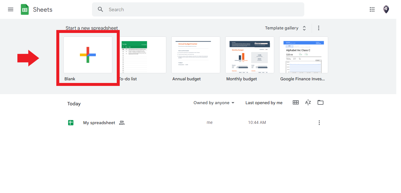
- Open a blank spreadsheet, or the file you already have.
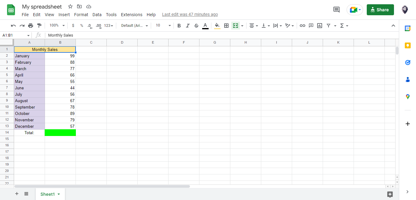
- Enter the numbers you want to total in a single column.
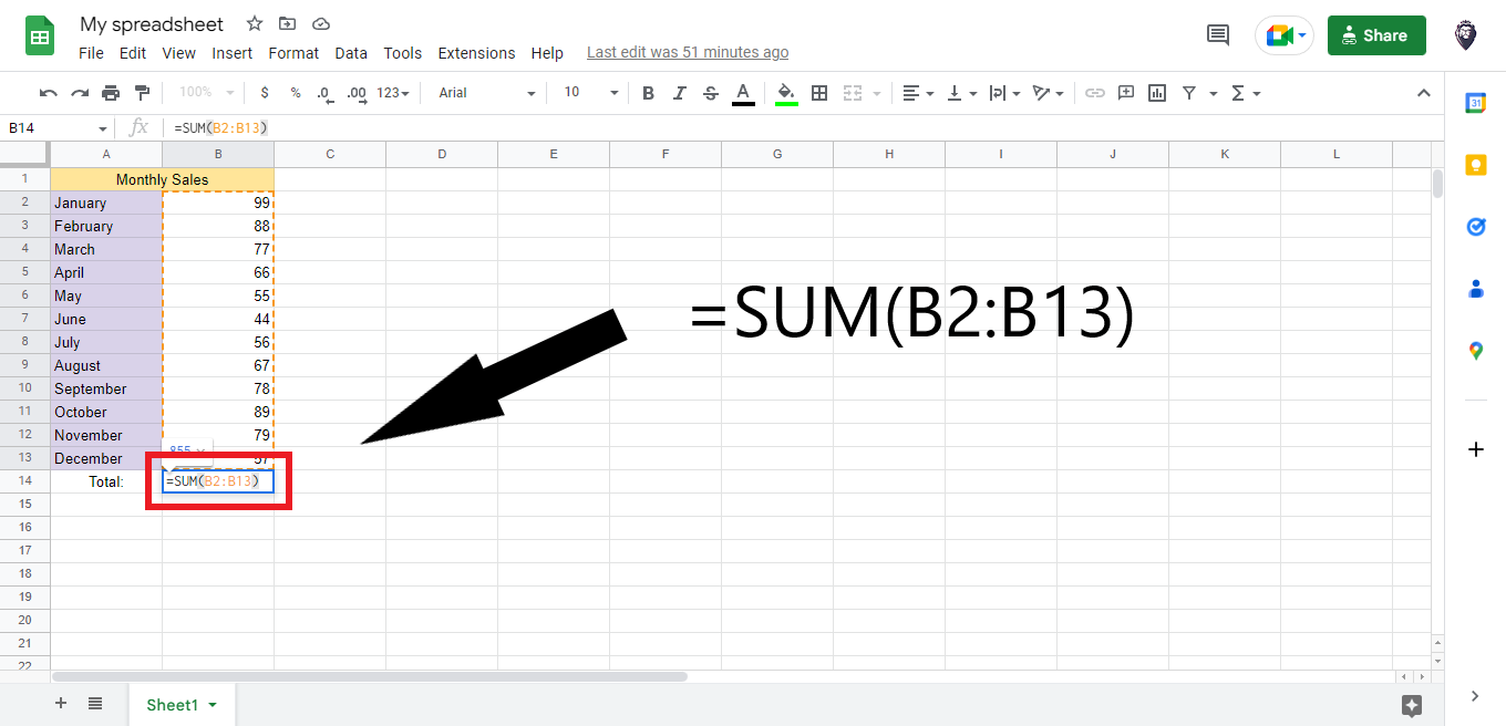
- Click an empty cell below the data, type
=SUM(and then drag over the cells you want to add. Sheets fills the range in for you as you drag.
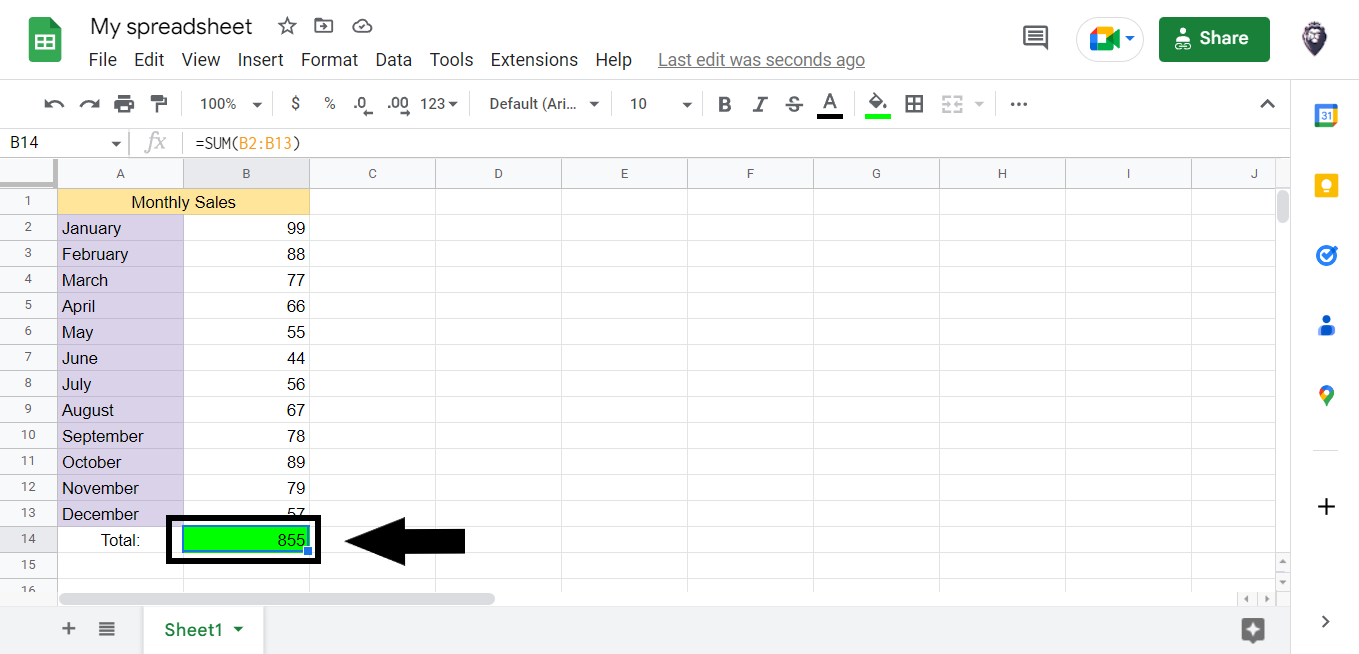
- Type the closing parenthesis and press Enter. The total appears in the cell, and the formula stays in the formula bar so you can edit the range later.
How do you sum an entire column that keeps growing?
Use an open-ended range. Leaving the end row off the reference tells Sheets to keep reading to the bottom of the sheet, so rows added next week are counted without you touching the formula.
Formula: =SUM(B2:B)
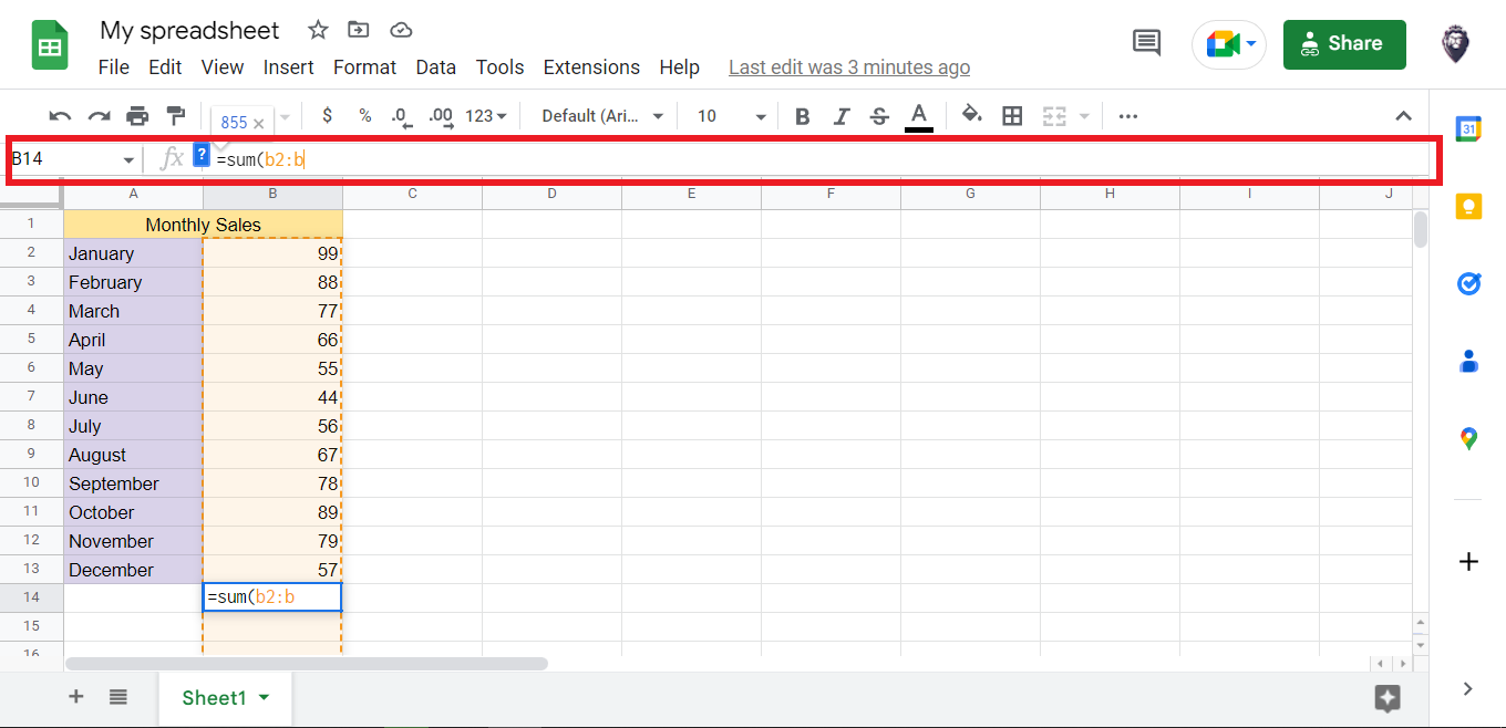
- Start at row 2, not row 1, so a numeric header such as a year is not swept into the total.
- Put the formula in a different column, or in a row above the data. If the total cell sits inside the range it is adding, Sheets returns a circular dependency error.
- If you must keep the total at the bottom of the same column, use a closed range that stops short of it, for example
=SUM(B2:B999)with the total in B1000.
The rule: an open range and a total cell can never share a column. One of them has to move.
How do you use AutoSum in Google Sheets?
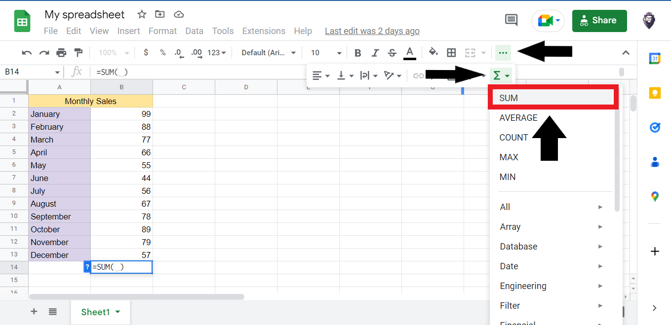
Google Sheets has an AutoSum equivalent in the toolbar, marked with the sigma symbol.
- Select the cells you want to add, or click the empty cell directly below them.
- Click the Σ (Functions) button on the right of the toolbar.
- Choose SUM from the list.
- Sheets guesses the range and highlights it. Adjust it by dragging if the guess is wrong, then press Enter.
Worth knowing: Google Sheets does not have Excel's Alt + = AutoSum shortcut, and plenty of tutorials repeat that claim incorrectly. Google's own keyboard shortcuts reference lists a different one: with a range selected, press Alt + Shift + Q on Windows or Option + Shift + Q on a Mac to jump to the quicksum in the status bar.
How do you see a column total without typing a formula?
Select the cells. The total appears in the status bar at the bottom right of the window, next to a small summary panel.
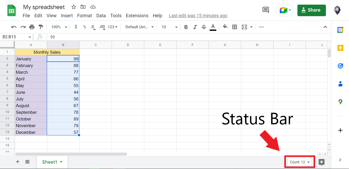
- Click that status bar figure to switch between Sum, Average, Min, Max, Count and Count numbers.
- Select a whole column by clicking its letter header to total everything in it at once.
- Hold
Ctrl(orCmdon a Mac) while selecting to total cells that are not next to each other.
The rule: the status bar is for reading a number once. Nothing is saved, nothing recalculates for anyone else, and nothing appears when you print. If someone else needs to see the total, it has to be a formula.
How do you sum only the rows that match a condition?
Use SUMIF for one condition and SUMIFS for two or more. Say column B holds invoice amounts, column C holds the status, and column D holds the client name.
| What you want | Formula |
|---|---|
| Total of every paid invoice | =SUMIF(C2:C, "Paid", B2:B) |
| Total of invoices over 100 | =SUMIF(B2:B, ">100") |
| Total of everything except one client | =SUMIF(D2:D, "<>Acme Ltd", B2:B) |
| Paid invoices for one client only | =SUMIFS(B2:B, C2:C, "Paid", D2:D, "Acme Ltd") |
| Total where the note contains "rush" | =SUMIF(E2:E, "*rush*", B2:B) |
Two details trip people up. SUMIF takes the range to test first and the range to add last, while SUMIFS reverses that and takes the range to add first. And a criterion that is not a plain value has to be a text string, so it is ">100" in quotes, never >100 on its own.
To compare a criterion against a cell instead of typed text, join them: =SUMIF(B2:B, ">"&F1) adds every value greater than whatever sits in F1.
How do you sum only the visible rows after filtering?
SUM has no idea a filter exists. It adds the hidden rows too. SUBTOTAL is the function that respects what is on screen.
Formula: =SUBTOTAL(109, B2:B)
The first argument is a function code that tells SUBTOTAL what to calculate and what to ignore.
| Formula | Rows removed by a filter | Rows you hid by hand |
|---|---|---|
=SUM(B2:B) |
Counted | Counted |
=SUBTOTAL(9, B2:B) |
Ignored | Counted |
=SUBTOTAL(109, B2:B) |
Ignored | Ignored |
The rule: use 109 unless you have a specific reason not to. It is the code that makes the total match what your eyes can see.
SUBTOTAL also skips other SUBTOTAL formulas inside its range, so nested group totals do not get double counted.
How do you sum the same column across several tabs?
List each sheet reference inside one SUM, separated by commas.
Formula: =SUM(January!B2:B, February!B2:B, March!B2:B)
- If a tab name contains a space, wrap it in single quotes:
=SUM('Q1 Sales'!B2:B, 'Q2 Sales'!B2:B). - Google Sheets does not support Excel-style 3D references such as
January:March!B2:B. Each tab has to be named individually. - To pull a total from a different file entirely, wrap IMPORTRANGE in SUM:
=SUM(IMPORTRANGE("spreadsheet_url", "Sheet1!B2:B")). You have to approve the connection once, the first time it runs.
How do you build a running total down a column?
Lock the start of the range and leave the end relative, then fill the formula down.
Formula in C2: =SUM($B$2:B2)
The dollar signs pin the first cell. As the formula copies down, C3 becomes =SUM($B$2:B3), C4 becomes =SUM($B$2:B4), and each row shows the cumulative figure to that point.
If you would rather write one formula that fills itself as data arrives, use an array version instead:
=ARRAYFORMULA(IF(B2:B="", "", SUMIF(ROW(B2:B), "<="&ROW(B2:B), B2:B)))
That leaves blanks blank and extends automatically down the column. Put it in C2 and leave the rest of column C empty.
Why is your sum returning 0 or the wrong number?
Almost every broken total comes from one of these seven causes.
| Symptom | Likely cause | Fix |
|---|---|---|
| SUM returns 0 | The numbers are stored as text, usually after a paste or CSV import. Text values sit left aligned in the cell. | Test one cell with =ISNUMBER(B2). If it says FALSE, select the column and use Data > Split text to columns to force Sheets to re-read the values, or total them with =ARRAYFORMULA(SUM(VALUE(B2:B100))). |
| Circular dependency error | The total cell is inside the range it is adding. | Move the total to another column, or close the range short of it. |
| Total ignores your filter | SUM counts hidden and filtered rows. | Swap to =SUBTOTAL(109, B2:B). |
| Total shows as a date or time | The result cell inherited date formatting from a neighbour. | Select the cell and choose Format > Number > Number. |
| Total is roughly double what it should be | An open range such as =SUM(B:B) is picking up another subtotal further down the column. |
Use =SUM(B2:B) and keep exactly one total cell per column, outside the range. |
| The formula displays as text | The cell is formatted as Plain text. | Set Format > Number > Number, then delete and retype the formula. |
| #VALUE! or #N/A in the total | One cell in the range holds an error, and SUM passes errors straight through. | Use =ARRAYFORMULA(SUM(IFERROR(B2:B, 0))), then go back and fix the broken cell. |
One more that is easy to miss: currency symbols and thousands separators typed by hand, such as $1,200 entered as text, make a cell unreadable to SUM. Enter 1200 and apply currency formatting instead of typing the symbol.
What if you are working in Excel instead?
The SUM function itself is identical, but the interface differs. Excel does have the Alt + = AutoSum shortcut, it has a built in Total Row for tables, and its SUBTOTAL codes behave the same way. If your file is an Excel workbook, start with how to add a total row in Excel.
Final thoughts
Most people only ever need =SUM(B2:B). The value in the rest of this guide shows up the day your total stops agreeing with your filter, or a pasted column silently adds to zero. Knowing which of the six methods matches the situation is what turns a spreadsheet from something you fight into something you trust.
You can visit our homepage for more easy-to-follow guides and Excel and Google Sheets templates.

Frequently asked questions
How do I total a column in Google Sheets automatically?
Put =SUM(B2:B) in a cell in a different column. The open ended range keeps reading to the bottom of the sheet, so every row you add later is included without editing the formula.
Is there an AutoSum shortcut in Google Sheets?
Not the Excel one. Alt + = does not trigger AutoSum in Sheets. Use the sigma button in the toolbar, or press Alt + Shift + Q with a range selected to jump to the quicksum in the status bar.
Why does my Google Sheets sum return 0?
The values are almost certainly stored as text rather than numbers, which is common after a CSV import. Check with =ISNUMBER(B2). If it returns FALSE, select the column and run Data > Split text to columns to convert them.
How do I sum only the rows my filter is showing?
Use =SUBTOTAL(109, B2:B). Plain SUM includes filtered out and manually hidden rows, so its total will not match what is on screen.
Can I sum the same column across multiple tabs?
Yes. Name each tab inside one formula, for example =SUM(January!B2:B, February!B2:B). Google Sheets does not support Excel style 3D references across a run of tabs.
Related Articles:
Basic Google Sheets Functions: What Are They and How to Use Them
The Top 5 Google Sheets Formulas You Need to Know
How to Subtract in Google Sheets

Want to Make Excel Work for You? Try out 5 Amazing Excel Templates & 5 Unique Lessons
We hate SPAM. We will never sell your information, for any reason.