The Must-Have Guide: How To Freeze A Row in Google Sheets

Are you constantly scrolling through your Google Sheets to find a specific row? 

You can mitigate this problem by freezing that particular row. This feature allows you to keep key pieces of data in place as you scroll around.

Today, we'll teach you how to freeze a row in Google Sheets so you can easily navigate through large datasets. You won't have to scroll endlessly to find important information.

Read on as we cover the following:

• When Would You Want to Freeze a Row in Google Sheets?

• Learn to Freeze Rows in Google Sheets

• Freeze Rows and Columns Using the Freeze Option

• Final Thoughts on How to Freeze a Row in Google Sheets

• Frequently Asked Questions on How to Freeze a Row in Google Sheets

When Would You Want to Freeze a Row in Google Sheets?

In several circumstances, you'll need to freeze single or multiple rows within Google Sheets. Here are some examples:

To keep content in one place

You can freeze a row to keep it in the same place.

Freezing a row means you can see that particular row no matter where you work in your spreadsheet.

You can freeze the rows or rows without scrolling to see information from a particular spreadsheet area. You will keep that information visible, so you don't have to keep scrolling up and down.

To make data entry easier

Another reason you may wish to freeze a row in Google Sheets is to make data entry easier.

If you are working on a big spreadsheet with lots of information, you must refer to the labels above the columns. That way, you can check the context of each column.

If you freeze the top row, you can keep your headings in view while entering data further down the spreadsheet.

Freezing a row will also improve the accuracy of data entry. After all, you'll lower the risk of entering data in the incorrect column.

To make a spreadsheet more reader-friendly

Another benefit of freezing a row or rows is making a reader-friendly spreadsheet.

Spreadsheets have a lot of rows and columns. It can be challenging to check everything if there is a lot of data.

If you freeze rows, you can refer back to them quickly as you navigate the rest of your spreadsheet.

To easily compare data

You can freeze a row in Google Sheets, so it is easier to compare different pieces of data.

It can be hard to remember what you found when looking at data from different parts of a big spreadsheet.

Freezing a row helps you save time. You will only need to spend time moving data around before you can start analyzing it. This way, you can focus on studying the data.

Learn to Freeze Rows in Google Sheets

Learning to freeze rows in Google Sheets is one of the important skills you'll need when you have a large data set. Here are some methods you can follow:

Freeze a row using the Freeze panes.

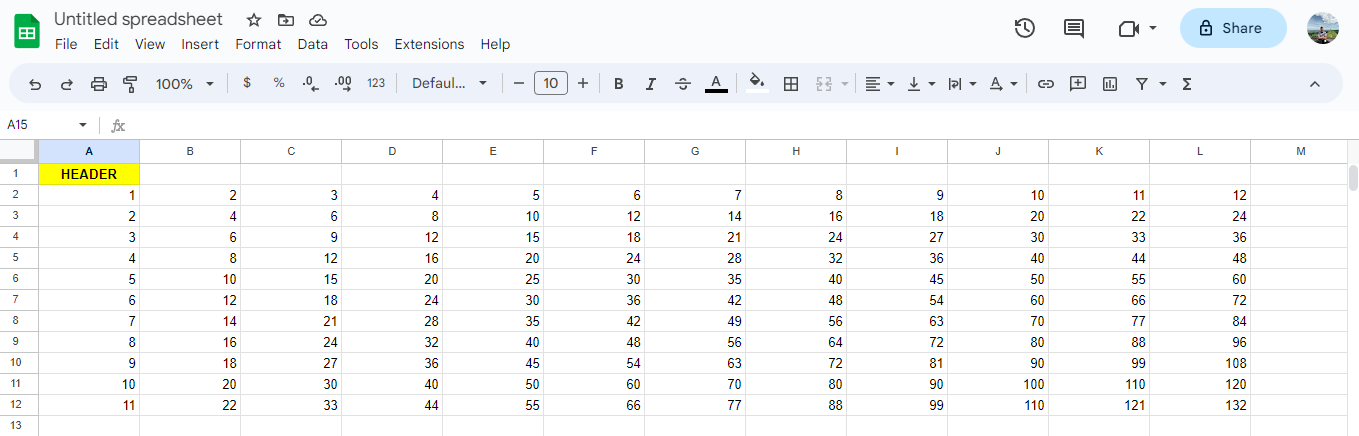
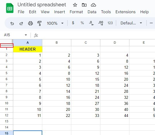
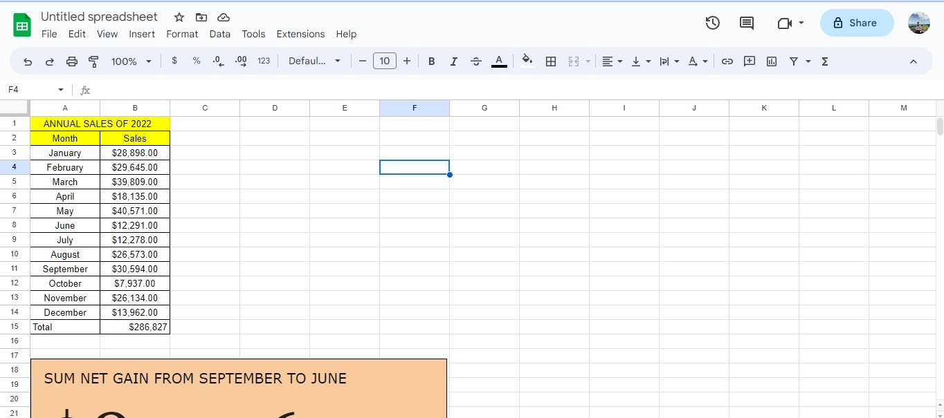
1. Open your Google Sheets spreadsheet.

2. Drag the Freeze pane to Row 1.

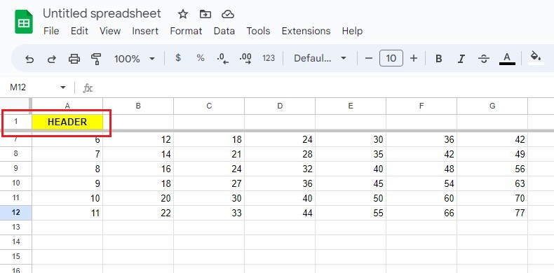
After following the steps above, Row 1 will be frozen in your spreadsheet. Moreover, you have learned to freeze a row in Google Sheets with Freeze Panes.

Freeze multiple rows using the Freeze panes.

Learn to freeze more than two rows using the Freeze panes feature by following the steps below:

1. Open your Google Sheets spreadsheet.

2. There are two thick gray lines, but drag the horizontal gray line to Row 2 of the spreadsheet or the key row.

   

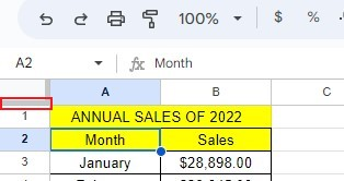
The rows above the thick gray line will be frozen in your spreadsheet. These rows will stay in place every time you scroll up and down.

Freeze Rows and Columns Using the Freeze Option.

To freeze rows and columns with ease using the Freeze option, follow the different methods below:

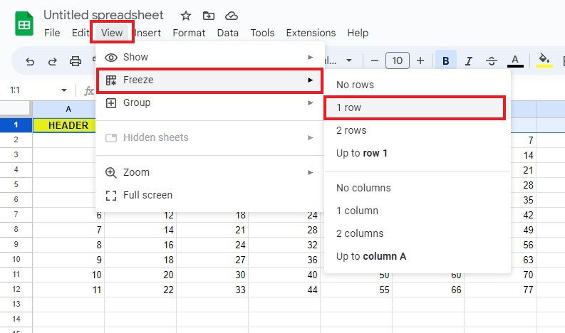
Freeze the first row in Google Sheets.

To have a frozen row in Google Sheets, follow the steps below:

1. Select a row you want to freeze.

2. Click the View menu, move your mouse to the Freeze option, and choose "1 row."

Freeze specific rows in Google Sheets.

To have frozen rows in Google Sheets, follow the steps below:

1. Select the last row of the selected rows you want to freeze.

2. Go to the View menu, move your mouse to the Freeze option, then choose "Up to row 4."

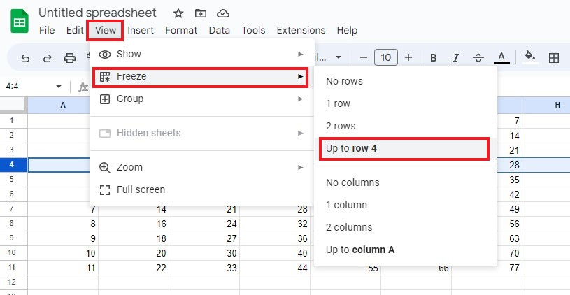
Following the steps above this will make selected rows frozen.

Freeze columns in Google Sheets.

To have frozen columns in Google Sheets, follow the steps below:

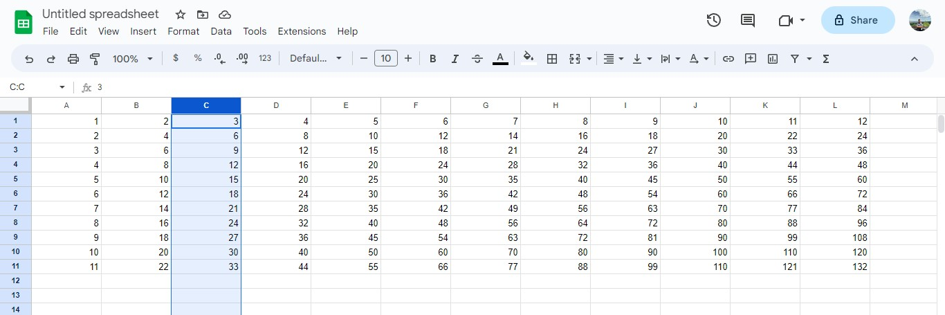
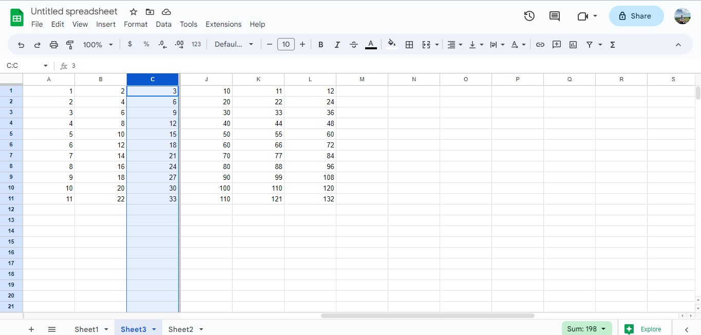
1. Select Column C to freeze Columns A to C.

2. Click the View menu, move your mouse to the Freeze option, then click "Up to column C."

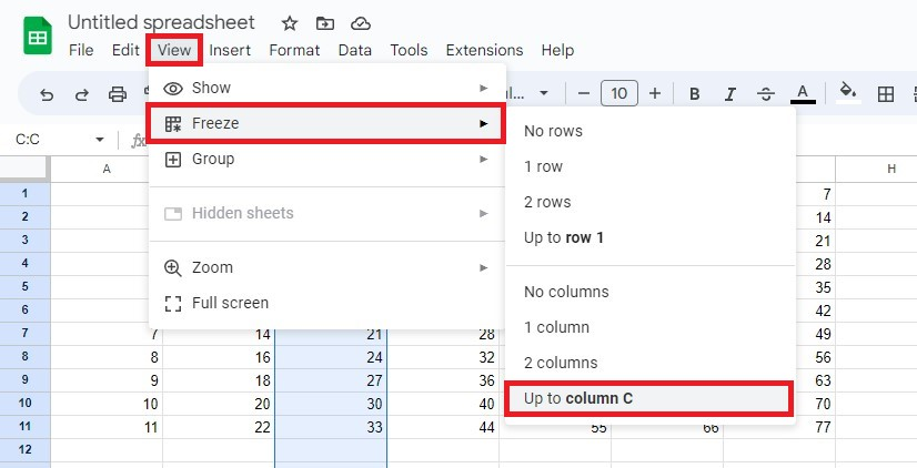
Following the steps above will make selected columns frozen.

Final Thoughts on How to Freeze a Row in Google Sheets

Simply freezing a header row keeps all your information aligned as you scroll through your document.

For more Google Sheets easy-to-follow guides and the latest Google Sheets templates, visit Simple Sheets now! There are also some other related articles on this topic below.

Don't forget to subscribe to Simple Sheets on Youtube for more easy-to-follow Google Sheets video tutorials!

Frequently Asked Questions on How to Freeze a Row in Google Sheets

Below are the most common questions about how to freeze a row in Google Sheets.

How do I freeze a specific row?

Select the row you wish to freeze, click View, and hover your mouse pointer over Freeze. Select the appropriate option from the context menu.

How do you freeze a row that isn't the first row of Google Sheets?

To freeze a row that isn't the first row:

1. Open your Google Sheets spreadsheet.

2. Select a row you want to freeze.

3. Go to the View menu, then move your mouse to the Freeze option.

4. Click "1 row."

Following the method below will freeze the selected row.

Can you freeze non-consecutive rows in Google Sheets?

You can freeze multiple rows that are non-consecutive within Google Sheets.

To freeze non-consecutive rows in Google Sheets, follow these steps:

1. Select the first row you wish to freeze.

2. Press and hold the CTRL or Command key, then select the second row you wish to freeze.

3. Repeat this to freeze multiple rows which are non-consecutive.

Repeat the same process to freeze columns or to unfreeze rows and unfreeze columns.

Related Articles:

How to Lock Cells in Google Sheets: Everything You Need to Know

How to Sort in Google Sheets: Quick and Easy Methods

How to Alphabetize in Google Sheets