Everything You Need To Learn About The Pivot Table In Excel

Are you looking to make the most of your new data and organization process?

Then you need to start utilizing pivot tables in Excel! Pivot tables are a fantastic tool that allows users to swiftly and easily sort, organize, and summarize large amounts of data within the same process as their spreadsheets.

Whether you're dealing with tons of raw material, want a better way to see sales value, or keep track of sales figures just for efficiency, this tool is invaluable!

Read on as we cover the following:

• Pivot Table in Excel

• Create Pivot Tables in Excel

• Final Thoughts on Pivot Table In Excel

• Frequently Asked Questions on Pivot Table In Excel

Pivot Table in Excel

The Excel Pivot Table is a tool to look at and summarize lots of data. It has powerful features that can help you analyze data related to totals and make reports showing the whole data set's meaning.

• Make large amounts of data easy to understand and navigate for the user.

• Categorize and subcategorize the data for summarization.

• Use filter, grouping, sorting, and conditional formatting techniques to narrow the data subsets and focus on the most important information.

• You can switch the rows to columns or columns to rows to see different information from your data. This is called "pivoting."

• Calculate the sum or total of numerical data in the spreadsheet.

• You can either expand or collapse the data levels and further delve into the details of any total by drilling down.

• Make a nice online version of your data or printed reports. Keep it short and eye-catching.

Create Pivot Tables in Excel

Many believe pivot tables are hard to make and time-consuming. But this isn't true! You can make your two-dimensional pivot table in just a few minutes.

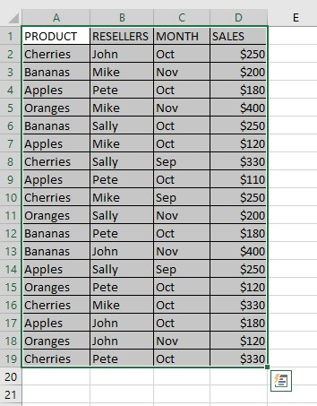
Prepare the source data.

Before summarizing sample data, organize your whole data set into columns and rows and convert your data range into an Excel Table. To do this:

1. Select your Pivot Table data.

   

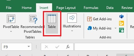
2. Navigate to the Insert tab, enter the Tables group, and click Table in Microsoft Excel.

3. Click on the OK button in the Create Table dialog box.

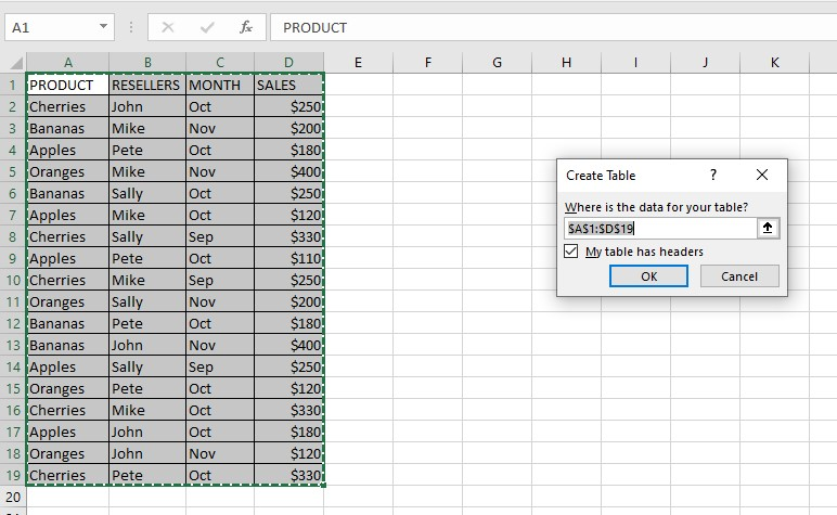
By using an Excel Table for your source data, you can enjoy the benefit of having a dynamic range, which means your table will automatically adjust its size as you add or remove entries or other data, ensuring that your Pivot Table is always up-to-date with the latest data.

Tips:

• When you make columns, give them unique, meaningful names. Later, these names will be the field names.

• Ensure that your source table has no empty rows or columns and does not include subtotals.

• To make maintaining your table easier, you can name your source table by going to the Design tab and entering the name into the Table Name box in the upper right corner of your worksheet.

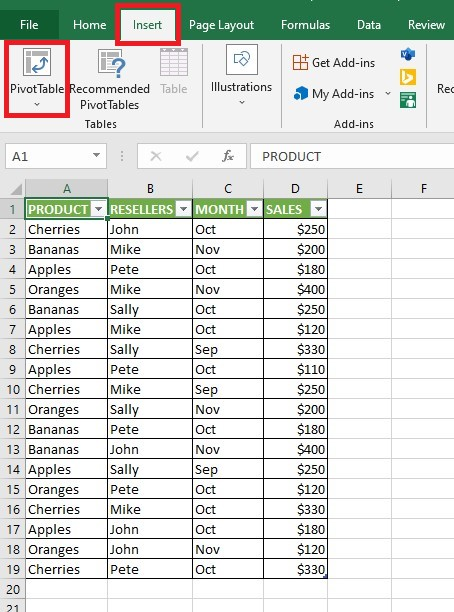
Insert a Pivot Table

1. Select a cell in the source data table, navigate to the Insert tab, and under the Tables Group, select PivotTable.

   

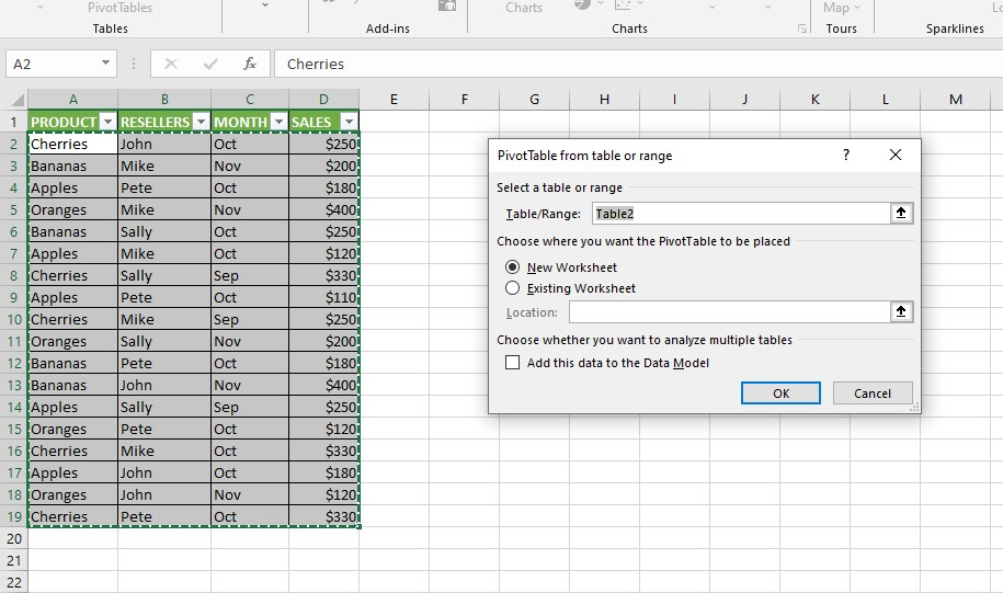
2. Select the range of cells in the data table, then choose a location for your Pivot Table.

3. After clicking OK, a blank Pivot Table resembling this created by Excel in the designated location.

Tips:

• Creating a new worksheet for the Pivot Table is usually better, especially for those new to it.

• Please specify the workbook and worksheet names when creating a Pivot Table using data from another worksheet or workbook.

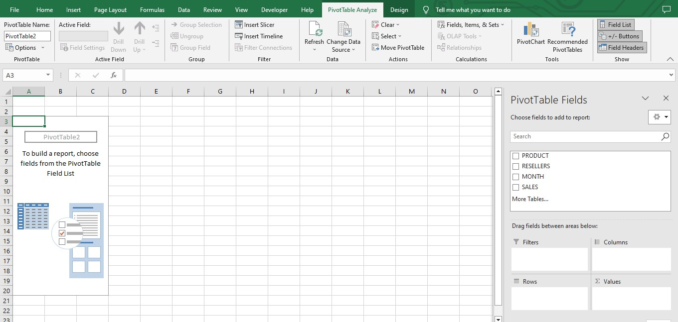
Adjust the layout of the Pivot Table report.

The section on the right-hand side of the worksheet where you can work with the fields of your summary report is the PivotTable Field List. They include headers and body sections.

The "Field Section" lists the available field names that you can include in your table. These field names will match the column names in your data source table.

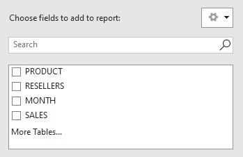
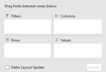
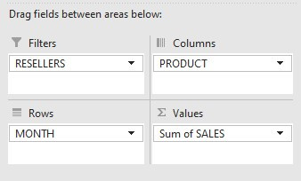
In the Layout Section, you will find the Report Filter area, Row Labels area, Column Labels, and Values area. You can use them to organize and show relevant information and adjust the fields in your table.

Any modifications to the PivotTable Field List, Excel will be instantly reflected in the table.

Insert a field into the Pivot Table.

To insert a field into the Layout section, check the box next to the field's name in the Field section.

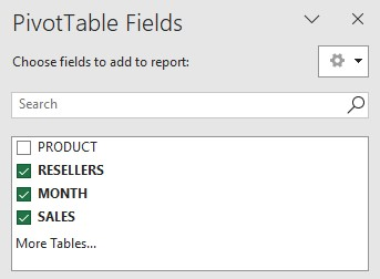
Microsoft Excel adds non-numeric fields to the rows area in the "Row Labels" area and numeric fields to the "Values" row area by default in the Layout section.

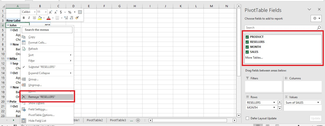
Delete a field from the Pivot Table.

You have two options to delete a specific field from your Pivot Table. First, you can uncheck the box next to the field's name in the "Field" section of the PivotTable pane.

Alternatively, you can right-click on the field within the PivotTable itself and click "Remove Resellers."

Organize the Pivot Table fields.

In the Layout section, you can change how the fields look in three ways.

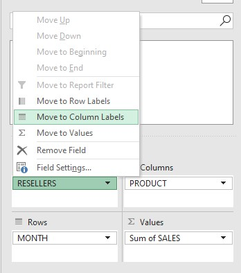
1. You can move fields between the four areas in the Layout section using your mouse. Another option is to click and hold the field name in the Field section and drag it to the desired area in the Layout section.

   Doing this will remove the field from its current location in the Layout section and place it in the new area.

   

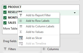
2. To add a field, right-click on its name in the "Field" section and choose the location where you want to place it.

   

3. To select the field and view its options, click on it in the Layout section.

Select a function for the Values field. (Note that this field is optional.)

Microsoft Excel automatically uses the SUM function for numeric values in the Values area of the Field List. Non-numeric data or blank values result in the COUNT function.

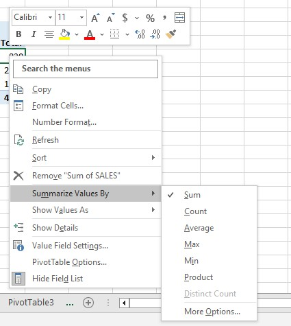
However, you can select a different summary function if desired. To do so in Excel 2013 and later versions, right-click the desired value field, select Summarize Values By, and then choose the desired summary function.

To learn more about the SUM function, check out How To Add In Excel in 4 Easy Ways in Simple Sheets now!

Add calculations in value fields.

One useful feature of Excel Pivot Tables is that they allow you to present values in various ways. For instance, you can display totals as percentages or arrange values from the column's area from smallest to largest and vice versa.

To access the "Show Values As" feature in Excel 2013 and higher, right-click on the field in the table. If you are using Excel 2010 and lower, you can find this option on the Options tab in the Calculations group.

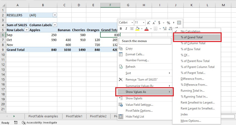
If you want to display total sales and sales as a percentage of the total for the same field, you can use the "Show Values As" function, which can be helpful if you have multiple instances of the same field. Here is an example table to illustrate this feature.

Do you know that you can remove the table formatting in Excel? Now, check out "How to Remove Table Formatting in Excel" in Simple Sheets!

Final Thoughts on Pivot Table In Excel

Learning the essentials of Pivot table creation in Excel can be a great way to help increase efficiency in data analysis. With the ability to sort, filter, and summarize information, working with data in Excel is much easier when using Pivot tables.

For more easy-to-follow guides, visit Simple Sheets and the Related Articles section of this blog post. Subscribe to Simple Sheets on Youtube for the most straightforward Excel video tutorials!

Frequently Asked Questions on Pivot Table In Excel

Can I make a Pivot table and Chart at the same time?

If you have Excel 2013 or a newer version, you can make a Pivot Table and Pivot Chart simultaneously.

1. Go to the Insert tab.

2. Then click Charts.

3. Then click the arrow under the PivotChart button and select PivotChart & PivotTable.

Can Excel refresh the Pivot Table Automatically every time I open my workbook?

Yes, Excel can refresh automatically update your Pivot Tables by doing these steps below:

1. Go to the "Analyze" tab

2. In the "PivotTable" group, click "Options."

3. In the "PivotTable Options" dialog box, go to the "Data" tab

4. Check the "Refresh data when opening the file" box.

5. Click the OK button.

Can I use any Interactive Pivot Table from the Pivot table layouts?

You can use a standard Pivot Table layout since a Pivot table is a tool that helps summarize large data sets and easily compare them interactively. It allows you to analyze numerical data and answer random questions about your data quickly.

Related Articles:

The Only Guide You Need About How To Multiply In Excel

Easiest Way To Learn How To Insert Pie Charts In Excel

Remove Blank Rows In Excel in 5 Easy Steps