
Learn How to Split Cells in Excel Quick and Easy
Feb 01, 2023
If you want to organize your data and make it easier to read, splitting cells in Excel is the way to go! Splitting cells allows you to separate one cell into multiple cells - perfect for separating first and last names, addresses, or any other information where each value needs its column.
This article will teach you how to split cells in Excel for an organized and accessible dataset. Get ready to say goodbye to messy spreadsheets forever!
Get our free Excel formulas cheat sheet
Plus new tutorials and template drops. Enter your email and we'll send it over.
Read more: How to unprotect a protected sheet in Excel
What Are Split Cells in Excel?
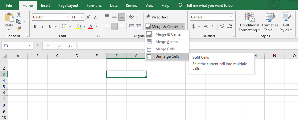
Splitting cells in Excel is a handy and powerful tool. With this feature, you can divide the contents of one cell across two or more cells rather than a standard single cell.
You can split cells horizontally – where the new cells are on the right of the original cell – or vertically, creating new cells beneath it. With split cells, you don't have words cut off mid-sentence—instead, split cells will get arranged in multiple adjacent cells in a compelling grid format.
Split cells in Excel allow a more organized look in your spreadsheet instead of unreadable and cluttered information. Split cells can also help keep long strings of words from spilling over into other columns and ruining their organization.
How To Split Cells in Excel Using the Text to Columns Wizard
Splitting cells in Excel using the Text to Column Wizard is a great way to separate information within cells into multiple columns. This feature discovers where data should be divided and helps ensure accuracy when organizing your Excel worksheet.
It's a powerful feature that can save you lots of time if you need to sort, organize, or analyze data from external sources.
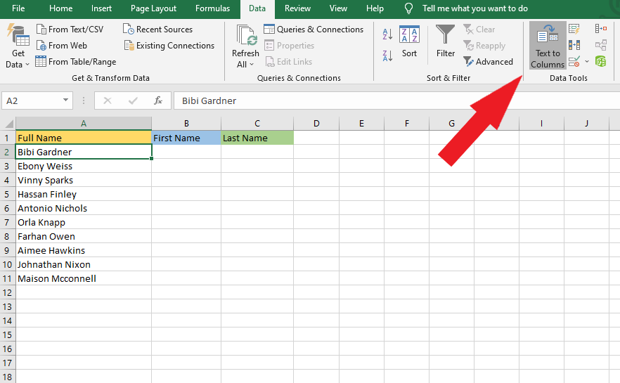
Step 1. Select a column you want to split the cells within.
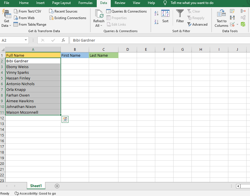
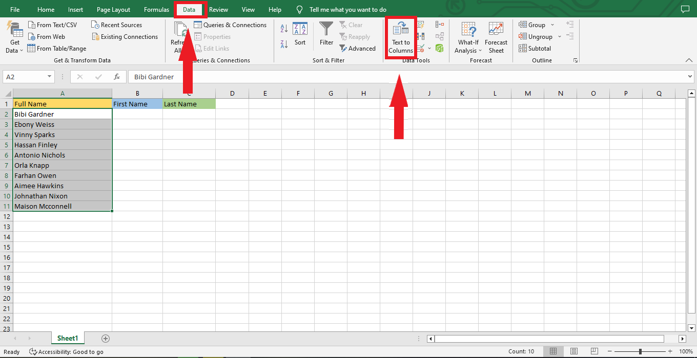
Step 2. Find the Text to Columns under the Data tab.
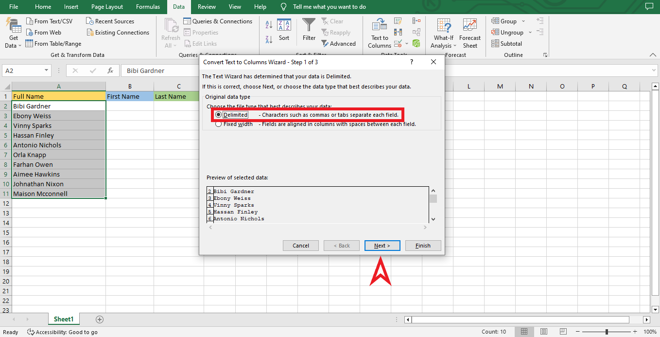
Step 3. A Convert Text to Columns Wizard opens. Select the Delimited option that best suits your data.
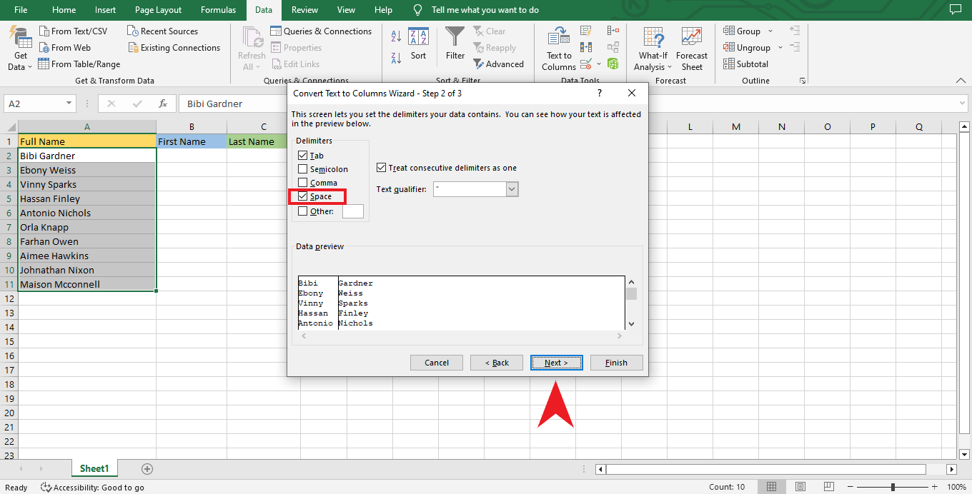
Step 4. In Convert Text to Columns Wizard Step 2 of 3, Choose "Space" as your Delimiter.
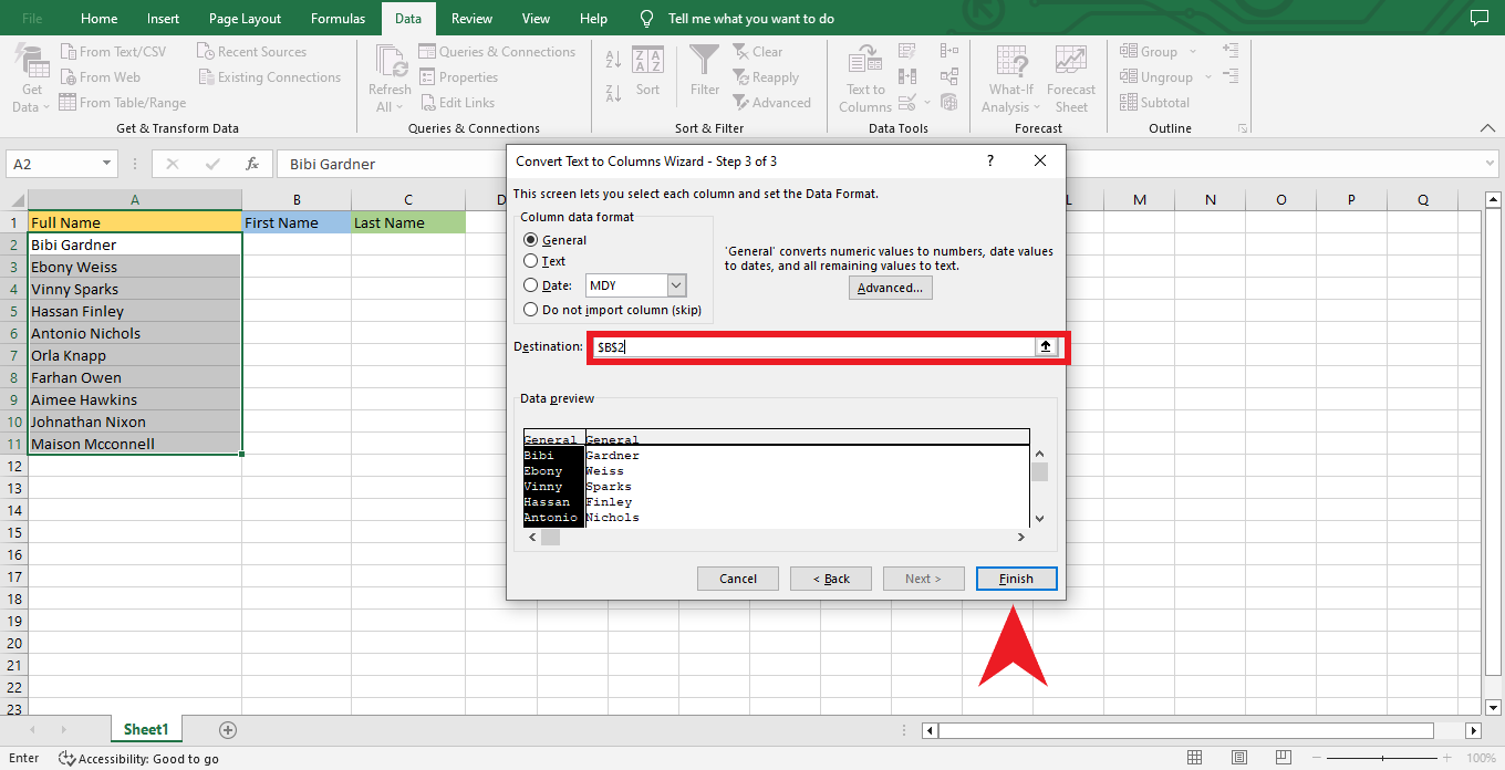
Step 5. Type your preferred destination cell in Convert Text to Columns Wizard Step 3 of 3.
For example: "=$B$2", always remember to leave sufficient space when multiple delimiters exist in your data.
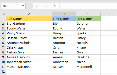
After you click "Finish," your selected cells have split into multiple cells using Text to Columns Wizard in Excel.
Note: Changing the names will not mirror the result column

Read more: How to connect slicers to multiple pivot tables.
How to Split Cells in Excel Using Flash Fill
Split cells in Excel using Flash Fill is a powerful tool for software users. Long-text entries can easily be divided into columns with this tool when needed.
It automatically looks for patterns in data that have been input and uses those to divide any individual cell data into multiple columns quickly. Splitting cells in Excel will save time as it eliminates the need to split every piece of information manually.
Flash fill also ensures no data is lost and all relevant information remains intact. Given this tool's usefulness, users of Excel should take advantage of it whenever possible.
Example 1:
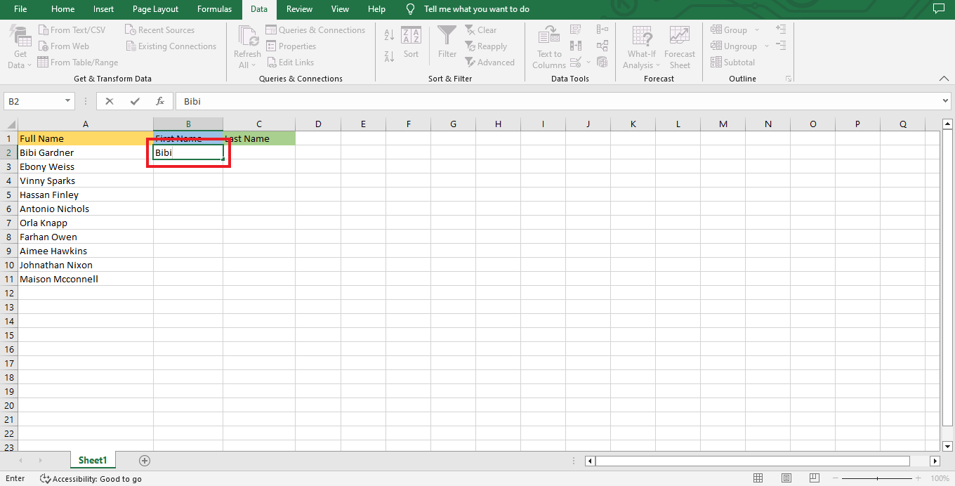
Step 1. To use the Flash fill option, type the first name in the second column.
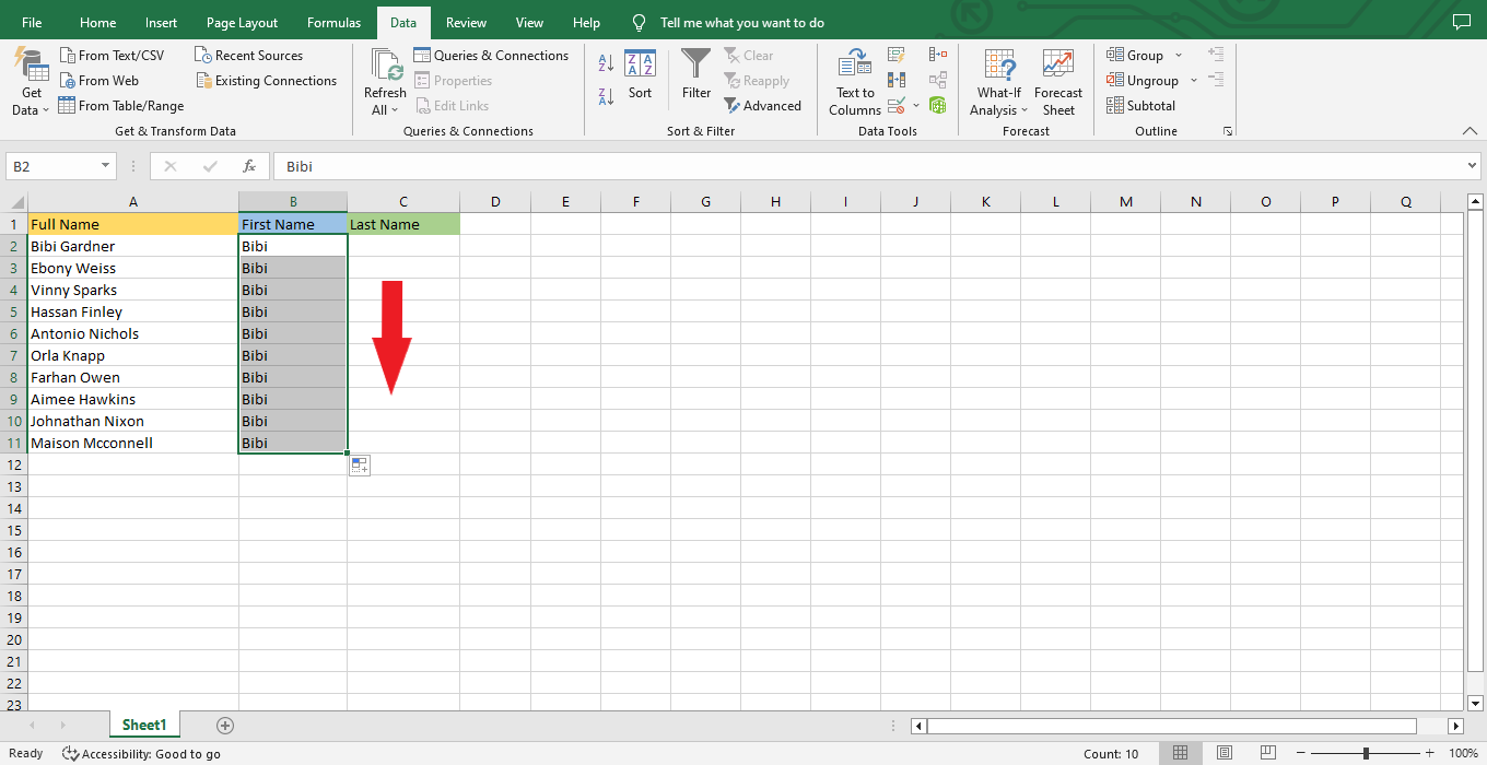
Step 2. Drag the fill handle to the last row of the data range.
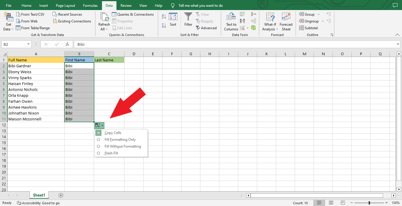
Step 3. Click the Auto Fill Options.
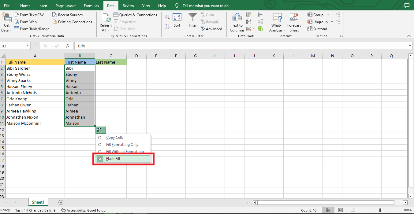
Step 4. Select Flash Fill, and you will notice that it fills the first names of the first column in column b.
The same steps apply when you want to fill the third column using the Flash Fill Option.
Example 2:
Here's another easy way to use Flash Fill Option.
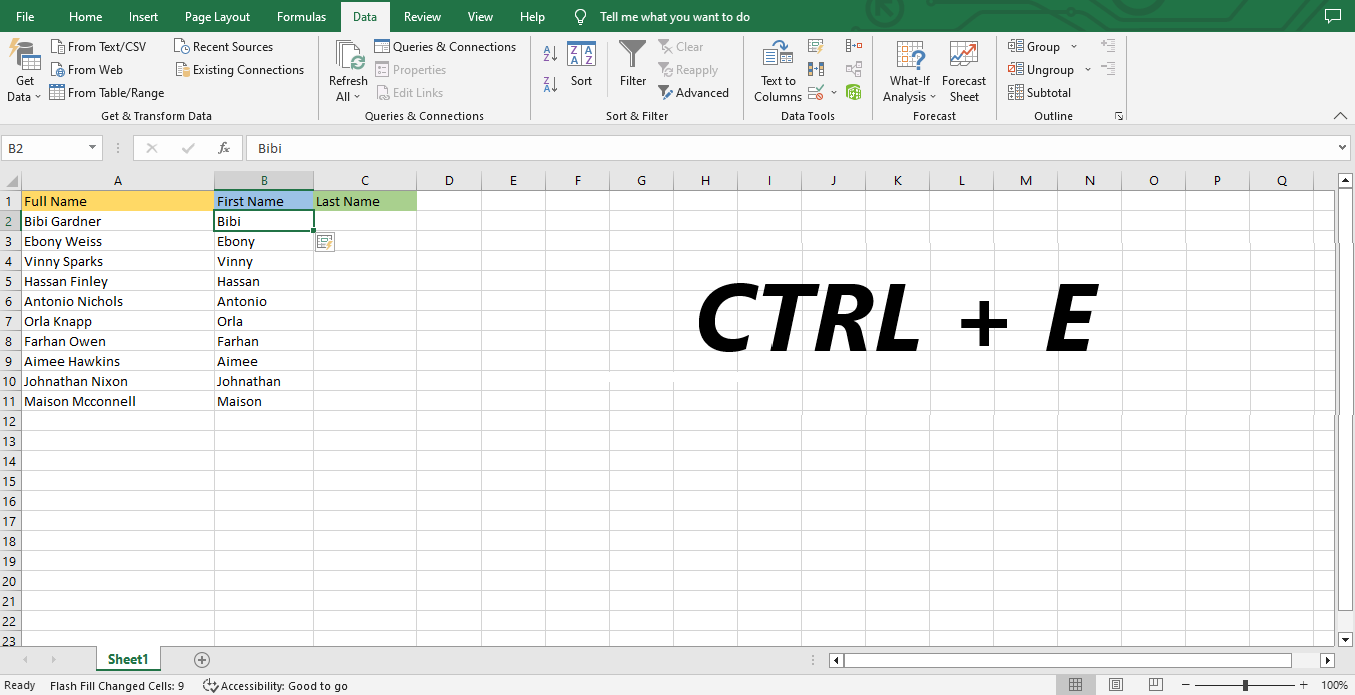
Step 1. Type the first name.

Step 2. Press CTRL + E to Flash Fill the column.
Read Also: How to Change Currency in Excel
How to split cells in Excel using Text Functions
A split cell in Excel using text functions is a convenient search function that can help you quickly get the information you need from a text string. Excel functions such as the left, right, and mid functions allow you to search and sort through text strings quickly and easily.
For example, if you have a text string containing a person's full name and address, you can use the left function to select just the name portion of the string to separate nicely within its cell. Split cells are beneficial for search functions when organizing large data sets; leveraging Excel's text functions makes data extraction even more accessible.
Example:
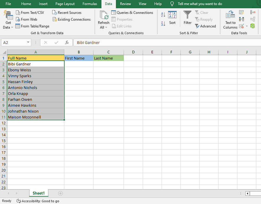
Step 1. Figure out the type of split you want to insert into the data. For ease of demonstration, I have chosen an example in which a single space separates the first and last names.
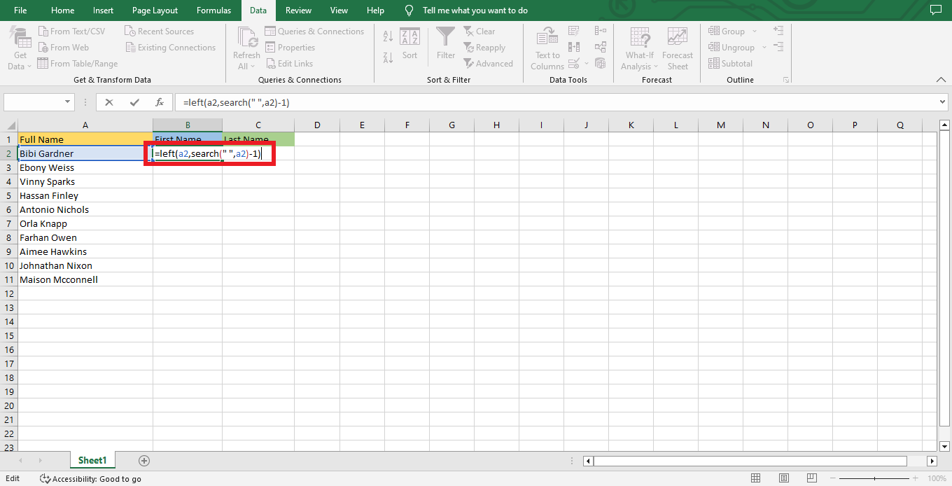
Step 2. Construct a combination to acquire the first name from a given source of SEARCH and LEFT functions.
Type the formula: =LEFT(A2,SEARCH(” “,A2)-1)
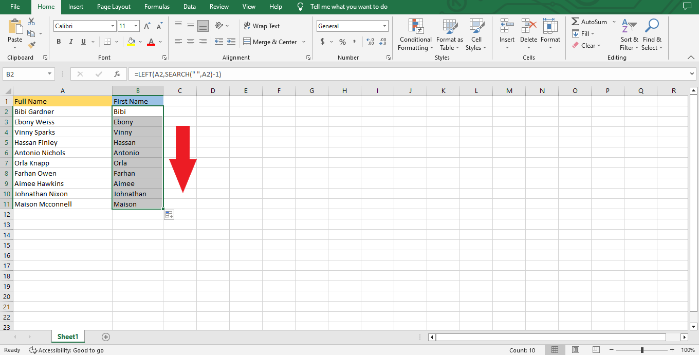
Step 3. Select the cell and copy where you type your formula, then drag the cursor down to the last range of your data.
To extract the last names, you need to replicate the same process. However, use the RIGHT function to retrieve data from the tail-end of each string.
Step 1. Type the formula =RIGHT(A2,LEN(A2)-SEARCH(” “,A2)) in cell C2.
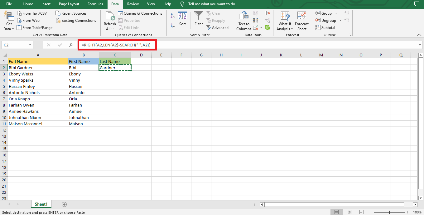
Step 2. Select the cell, copy where you type your formula, then drag the cursor down to the last range of your data.
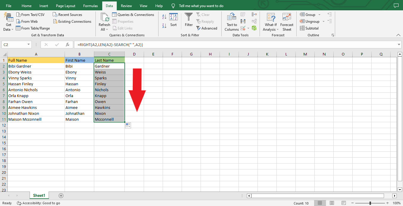
Well done! You have successfully split the first and last names.
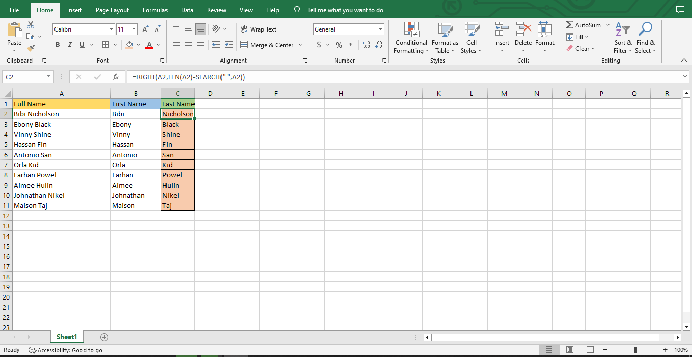
It is essential to highlight that the split is dynamic; in other words, when you modify the source data, your results are automatically adjusted.
Read more: How to convert PDF to an Excel spreadsheet.
How To Split Cells in Excel Using Power Query
Example:
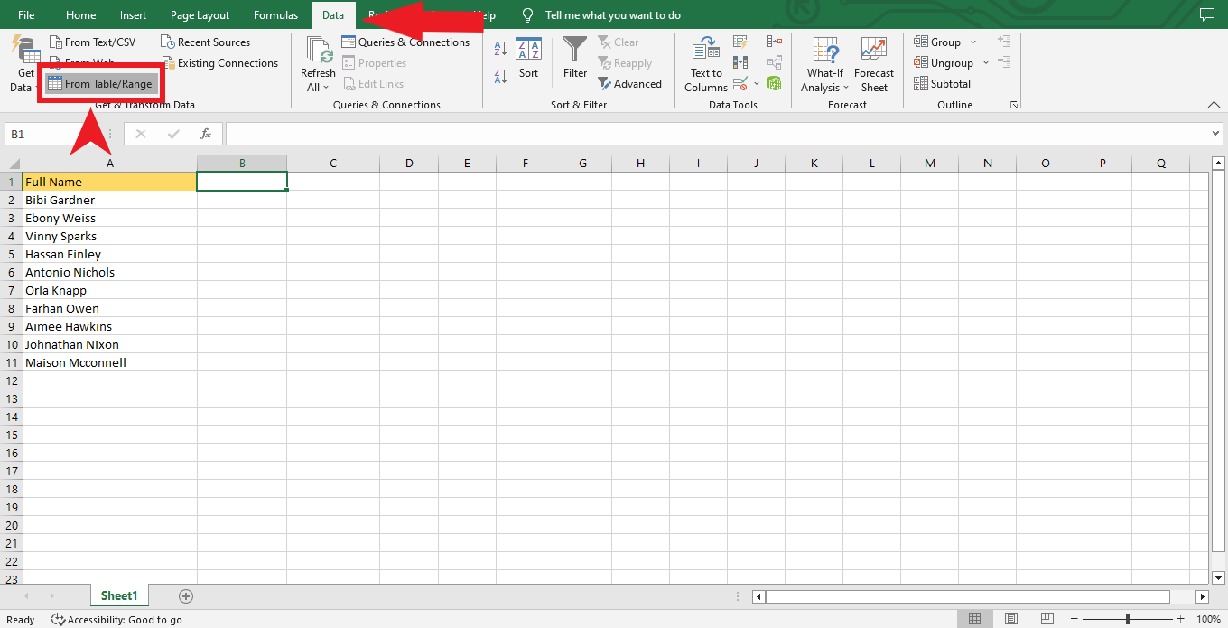
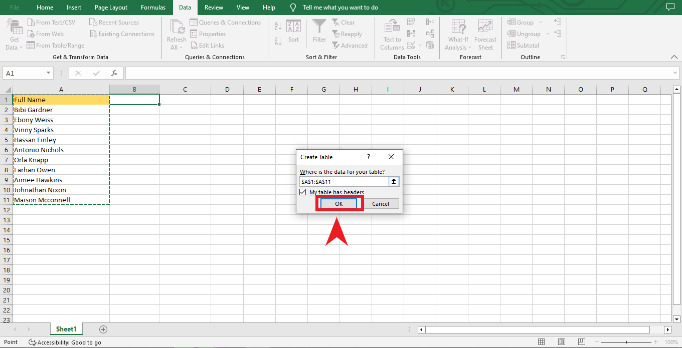
Step 1. To begin, select a cell within your data set, then navigate to the ribbon and click Data (tab) > From Table/Range or Data(tab)>From Sheet for more recent versions of Excel.
Step 2. A Create Table window will pop up if your chosen cell isn't part of an Excel table. Ensure that all rows and columns are joint in your selection, and ensure the "My table has headers" option is checked before clicking OK.
Step 3. Open the Power Query editor to reveal all your data, then navigate to Home > Split Column (drop-down) on the ribbon and select By Delimiter to get started.
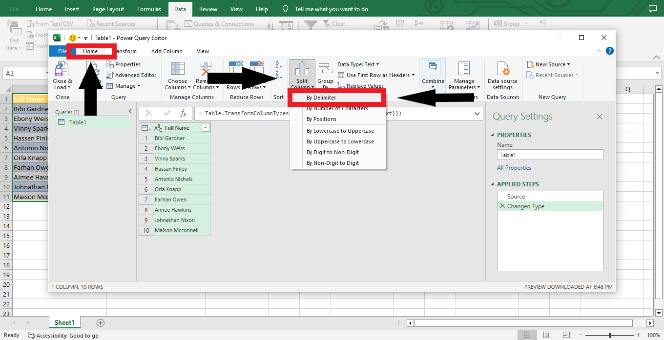
Step 4. Multiple methods divide cell contents by various positions depending on the length of your text. In our example, both a space and each instance of the separating character make good selections. Click OK to complete.

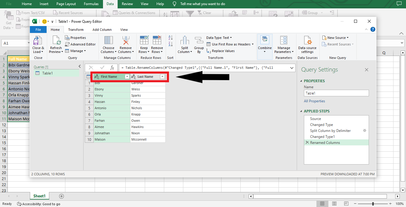
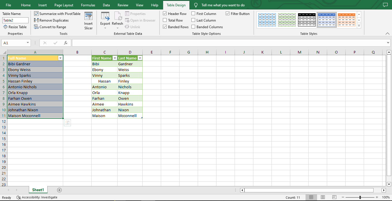
Step 5. Now, in the data preview window, you can see that the names have got divided into two columns. To make it easier to identify them, double-click on the header and rename it from "First Name" and "Last Name," respectively.
Step 6. Now, it is time to export the data back into Excel. To do this, select Home > Close & Load (drop-down) followed by selecting "Close & Load To..."
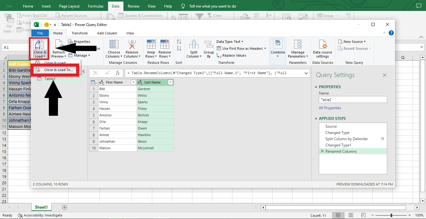
Step 7. Select Table from the Import Data dialog box and choose where to load the information. In the example, I have selected an existing sheet at cell C1. Click OK.
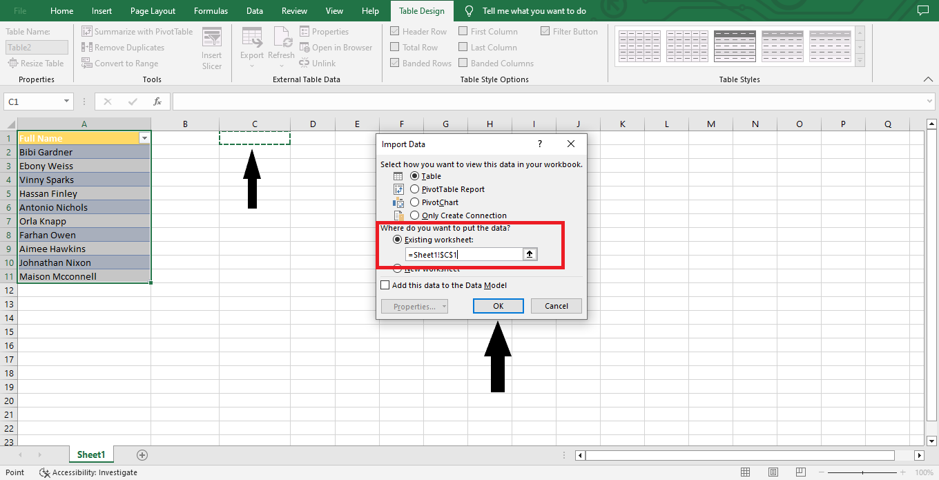
The new Power Query data will be included in the Excel cells for easy viewing.
Read Also: The Easiest Way to Connect a Slicer to Multiple Pivot Tables in Excel
Note:
-
For new updates to our source cells or additional names, we can click Data > Refresh All, and the outcome will be new!
-
Following this process will transform your source cells into an Excel table.
-
Power Query can deliver with its Column from Examples feature if you require more advanced capabilities than simple delimiter-based splitting. Power Query allows sophisticated string manipulation and transformation in a few easy steps.
Conclusion
Now you have four methods to help you split cells in Excel. As you can see, each method has its advantages and purposes, so be sure to choose the one best suited to your needs.
Frequently Asked Questions:
What are split cells in Excel?
Split cells in Excel are a handy feature for sorting and organizing data. With split cells, you can have text in one cell divided across two or more adjacent cells - all of which will be connected correctly to the original cell.
How do I split cells in Excel?
Select the cell or cells you want to split and click 'Data' on the menu toolbar to do this. Here, you will find the option 'Text to columns,' which allows you to divide your text into separate cells based on specific criteria like a particular character or spacing.
What are some of the benefits of using split cells in Excel?
With split cells, rows and columns are divided into smaller sections to highlight the differences between values in a single cell. This feature allows users to categorize information better while organizing it in the same space.

Related Articles:
Want to Make Excel Work for You? Try out 5 Amazing Excel Templates & 5 Unique Lessons
We hate SPAM. We will never sell your information, for any reason.

