How to Wrap Text in Excel: Shortcuts, Merged Cells and Fixes
Jan 21, 2026
Short answer: how do you wrap text in Excel?
To wrap text in Excel, select the cells, then click Home > Wrap Text, or press Alt, then H, then W. Excel breaks the text onto extra lines inside the same cell and grows the row height to fit. If the row does not grow, the row height is fixed or the cells are merged.
Last updated: August 18, 2026
Get our free Excel formulas cheat sheet
Plus new tutorials and template drops. Enter your email and we'll send it over.
Table of Contents
- How do you wrap text in Excel? Three methods
- Wrap Text vs Shrink to Fit vs manual line break
- Why is wrap text not working in Excel?
- How do you wrap text in merged cells?
- How do you wrap a whole column instead of one cell?
- How do you wrap text inside a formula result with CHAR(10)?
- How do you stop text overflowing without wrapping it?
- How does wrap text behave in Tables and PivotTables?
- How do you print wrapped text without cutting it off?
- How do you make wrap text the default?
- Frequently asked questions

How do you wrap text in Excel? Three methods
Wrap Text is a display setting. It tells Excel to break a long entry onto extra lines inside the same cell instead of spilling it across neighbouring columns or cutting it off. The underlying value never changes, which is why the formula bar still shows one continuous string.
Rule: Wrap Text changes how a cell looks, never what it stores. Only Alt + Enter actually writes a character into the cell.
Method 1: the Wrap Text button on the ribbon
-
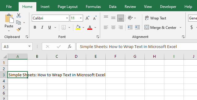
Select the cell or range that holds the long text.
-
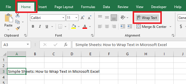
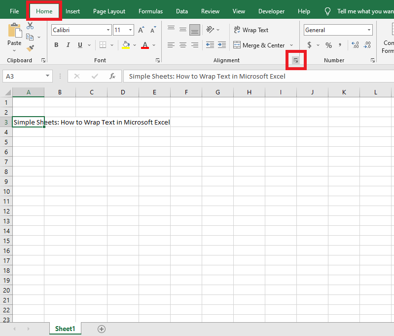
Go to the Home tab, find the Alignment group, and click Wrap Text.
-
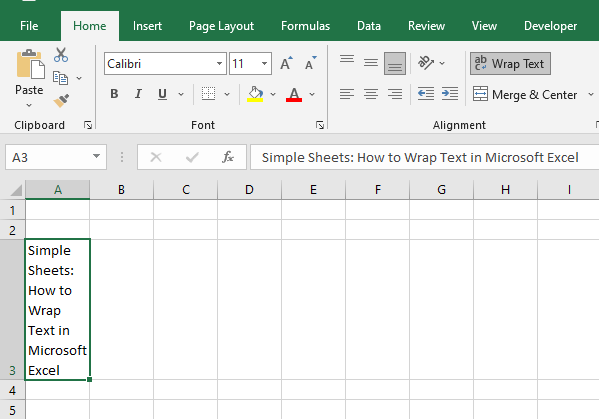
Excel wraps the text and autofits the row height so every line is visible.
Keyboard shortcut: on Windows, press Alt, release it, then press H, then W. It is a ribbon sequence, not a held combination. On Mac there is no built in shortcut for the Wrap Text toggle, so either use the ribbon or create a custom app shortcut in System Settings.
Method 2: the Format Cells dialog
Use this when you want to set wrapping, alignment and indent in one pass, or when you are formatting a large range.
-
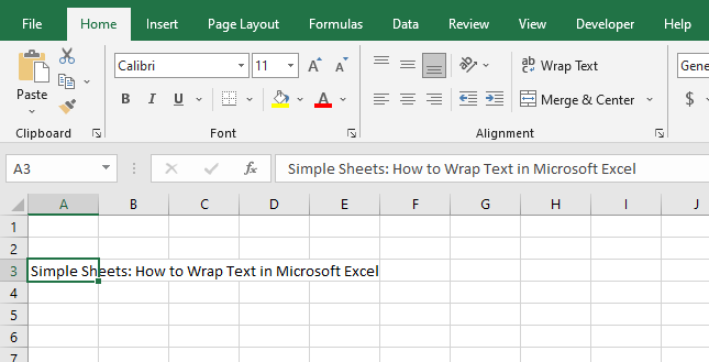
Select the cells you want to format.
-
Press Ctrl + 1, or click the small Alignment Settings arrow on the Home tab.
-
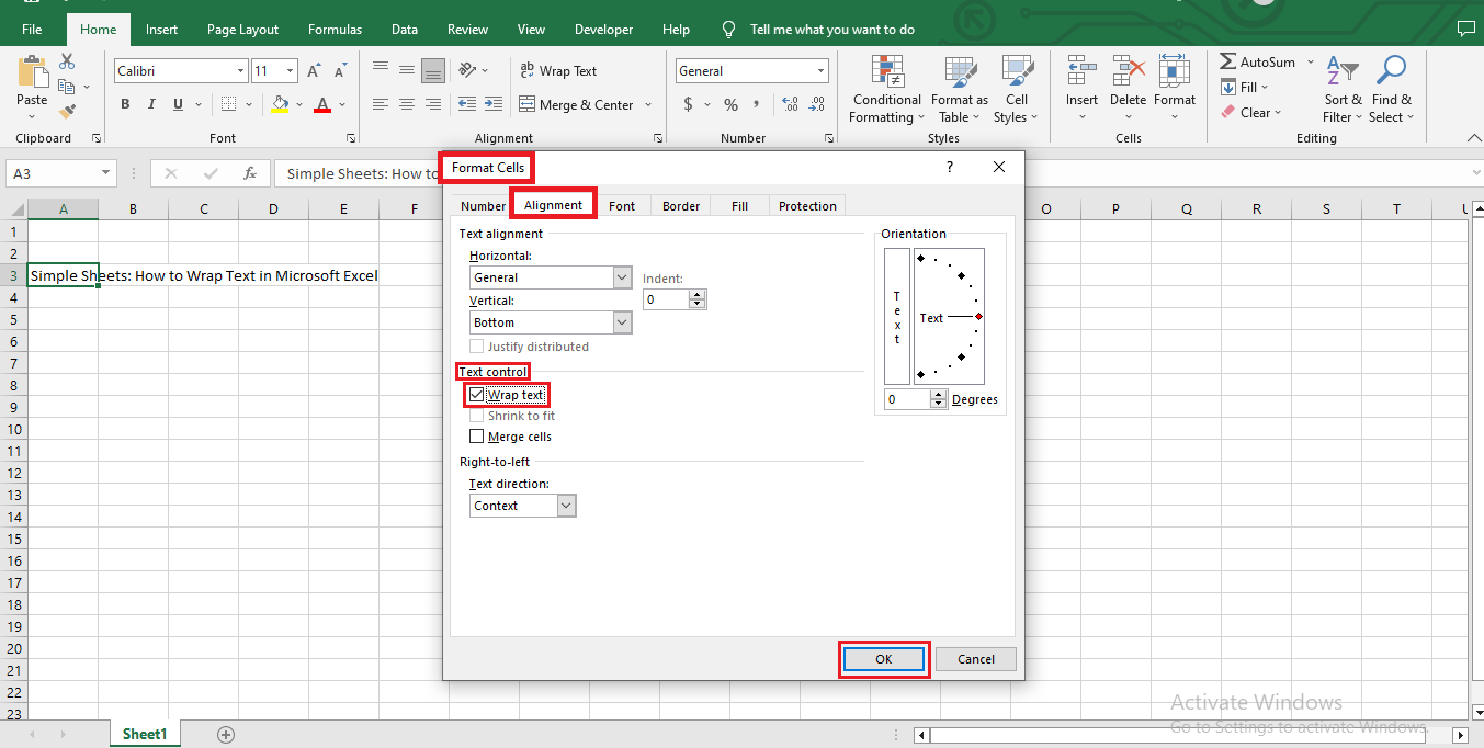
In the Alignment tab, under Text control, tick Wrap text and click OK.
-
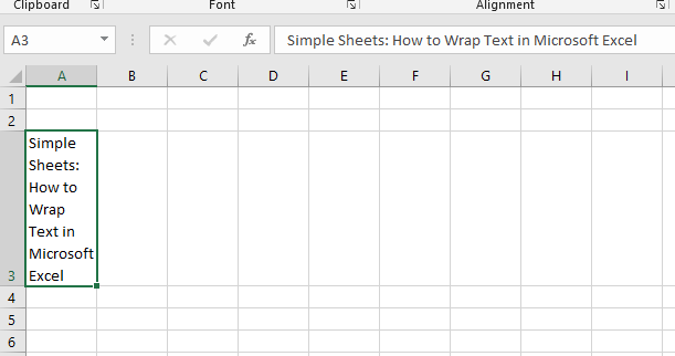
The rows resize to show the wrapped text at the current column width.
Microsoft documents the same two routes in its official guide, Wrap text in a cell in Excel.
Method 3: force the break yourself with Alt + Enter
Automatic wrapping breaks lines wherever the column edge happens to fall. When you need the break in an exact place, such as between the street and the city of an address, insert a hard line break instead.
-
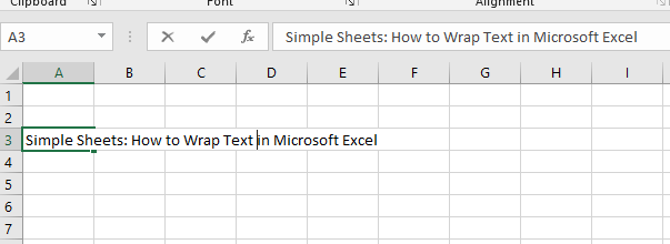
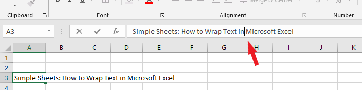
Double-click the cell, or press F2, to get into edit mode.
-
Click the exact spot where you want the new line to start.
-
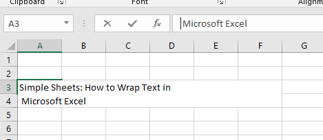
Press Alt + Enter on Windows, or Control + Option + Return on Mac.
-
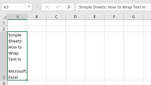
The entry splits at that point and stays split no matter how wide the column gets.
If you work with manual line breaks a lot, our deeper guide covers finding, removing and replacing them: How to start a new line in an Excel cell.
Wrap Text vs Shrink to Fit vs manual line break
These three options all deal with text that is too long for its column, and they behave completely differently. Wrap Text and Shrink to Fit are mutually exclusive: ticking one clears the other.
| Behaviour | Wrap Text | Shrink to Fit | Manual break (Alt + Enter) |
|---|---|---|---|
| What it does | Flows the text onto extra lines in the same cell | Shrinks the displayed font size until the text fits on one line | Splits the entry at the exact point you choose |
| Where the break falls | Wherever the column edge lands | No break at all | Exactly where your cursor was |
| Changes row height | Yes, autofits unless the height is fixed | No | Yes, once Wrap Text is on |
| Changes the stored value | No | No | Yes, it inserts CHAR(10) into the cell |
| If you resize the column | Text re-flows | Font rescales | The break stays put |
| Best for | Notes, descriptions, long column headers | Short codes and IDs in narrow columns where row height must stay fixed | Addresses and multi-line labels that must always break in the same place |
Rule: if the layout must never change, use a manual break. If the layout should adapt to the column, use Wrap Text. Never expect both Wrap Text and Shrink to Fit at once, Excel only honours one.
Read Also: How to Add a Signature in MS Excel?
Why is wrap text not working in Excel?
This is the most common wrapping complaint, and it is almost never a bug. Wrap Text is switched on, but something is stopping the row from growing tall enough to reveal the extra lines. Work through these causes in order.
1. The row height has been set manually
Once you drag a row border, Excel marks that row as a fixed height and stops autofitting it forever. Wrapped lines two and three are there, they are just hidden below the visible band.
Fix: select the row, then click Home > Format > AutoFit Row Height, or double-click the bottom border of the row header.
2. The cells are merged
AutoFit Row Height does not work on merged cells. Excel will wrap the text but it will not calculate a new height for you.
Fix: drag the row height manually, or unmerge and use Center Across Selection instead. See the merged cell section below.
3. Shrink to Fit is switched on
Shrink to Fit and Wrap Text cannot both apply to the same cell. If Shrink to Fit was set earlier, ticking Wrap Text may look like it did nothing.
Fix: press Ctrl + 1, go to the Alignment tab, and clear the Shrink to fit checkbox before ticking Wrap text.
4. Vertical alignment is hiding the extra lines
If the row is taller than one line but the cell is bottom aligned or top aligned inside a very tall row, the wrapped lines can sit outside the part of the row you are looking at.
Fix: set vertical alignment to Top, then autofit the row height.
5. You have hit the 409 point row height ceiling
A single Excel row cannot be taller than 409 points, which is roughly 545 pixels. Very long entries, such as a pasted paragraph, will wrap but the tail will be invisible because the row physically cannot grow any further.
Fix: widen the column, reduce the font size, or split the entry across several cells.
6. The sheet is protected
If the Wrap Text button is greyed out, the worksheet is protected and cell formatting is not an allowed action.
Fix: use Review > Unprotect Sheet, change the formatting, then re-protect.
Rule: if wrapped text is invisible, the problem is row height nine times out of ten. Check for a manually dragged row or a merged cell before you touch anything else.
How do you wrap text in merged cells?
You can absolutely apply Wrap Text to a merged cell. The catch is that Excel will not autofit the height of a row containing merged cells, so the wrapped lines stay hidden until you resize the row yourself.
You have three practical options:
- Wrap and drag. Apply Wrap Text, then drag the bottom border of the row header down until every line shows. Fine for a title row you set once.
- Use Center Across Selection instead of merging. Select the cells, press Ctrl + 1, go to Alignment, and set Horizontal to Center Across Selection. The text looks centred across the range, the cells are never actually merged, and AutoFit Row Height starts working again.
- Unmerge, then re-plan the layout. Merged cells also break sorting, filtering and many formulas, so if a sheet is going to be worked in rather than just printed, unmerging is usually the right call.
Rule: Center Across Selection gives you the look of a merged heading with none of the autofit, sorting or formula problems.
Related: How to Merge Cells in Excel
How do you wrap a whole column instead of one cell?
Wrap Text is cell formatting, so it applies to whatever you have selected when you click it. Choosing the right selection is what makes it stick for future rows.
| What you want | What to select first | Applies to new rows? |
|---|---|---|
| One cell | The cell | No |
| A fixed block of data | The range, for example B2:B500 | Only inside that range |
| An entire column | The column header letter | Yes, anywhere in that column |
| Several non-adjacent columns | Ctrl-click each column header | Yes |
| A growing data set | Convert to a Table with Ctrl + T, then format the column | Yes, the Table extends the format |
| The whole sheet | Ctrl + A, or the corner box | Yes, but it slows large files down |
You can also copy the formatting alone. Format one cell the way you want it, click Format Painter on the Home tab, then drag across the target range. Double-click Format Painter to keep it active for multiple ranges.
Rule: select the column header, not the used range, if you want wrapping to apply to rows that do not exist yet.
How do you wrap text inside a formula result with CHAR(10)?
Wrap Text will not break a formula result on its own, because the result is a single string with no break characters in it. To force a line break inside a formula you have to build the break into the text using CHAR(10) on Windows, or CHAR(13) on Mac.
Join a name and an address onto separate lines:
=A2&CHAR(10)&B2&CHAR(10)&C2
Or with TEXTJOIN, which is cleaner when you have several parts and some may be blank:
=TEXTJOIN(CHAR(10),TRUE,A2,B2,C2)
Two things trip people up here:
- Wrap Text must be switched on for the result cell. Without it,
CHAR(10)is still in the string but Excel renders it as a single line, and you will see nothing change. - The break character is invisible. If you later need to strip breaks out, use
=SUBSTITUTE(A2,CHAR(10)," "), or use Find and Replace and type Ctrl + J into the Find field to represent the line break.
Rule: CHAR(10) supplies the break and Wrap Text reveals it. You need both, and a formula that looks broken is almost always missing the second one.
How do you stop text overflowing without wrapping it?
Sometimes you do not want taller rows at all, you just want long entries to stop spilling across the columns to the right. Wrapping is the wrong tool for that. Use alignment instead.
- Select the cells and press Ctrl + 1.
- Go to the Alignment tab.
- Open the Horizontal dropdown and choose Fill, then click OK.
The text is now clipped at the cell border. Row height does not change, nothing spills into the neighbouring column, and the full value is still there in the formula bar. Typing anything at all into the cell to the right has the same clipping effect, which is why overflow often looks inconsistent across a sheet: it depends on whether the next cell is empty.
Rule: text only spills into the next column when that column is empty. Horizontal alignment set to Fill clips it permanently without changing row height.
How does wrap text behave in Tables and PivotTables?
Excel Tables (Ctrl + T) handle wrapping well. Format the column once and every new row you add inherits the wrapping automatically. This is the cleanest way to keep a growing log or tracker readable.
PivotTables fight you, because they re-apply their own layout every time they refresh. Wrap a PivotTable header, refresh, and the column snaps back. The fix is a PivotTable option, not a cell format:
- Right-click anywhere in the PivotTable and choose PivotTable Options.
- On the Layout & Format tab, clear Autofit column widths on update.
- Tick Preserve cell formatting on update.
- Click OK, then apply Wrap Text and set your column widths.
Rule: wrapping in a PivotTable will not survive a refresh until you clear "Autofit column widths on update" in PivotTable Options.
Related: How To Add a Drop-down List in Excel?
How do you print wrapped text without cutting it off?
Wrapped text that looks perfect on screen often prints with the last line sliced off. That happens because Excel prints the row at its stored height, and a screen row that was quietly autofitted can be taller than the printed band.
- Autofit before printing. Select all rows, then Home > Format > AutoFit Row Height. This alone fixes most cut-off lines.
- Add a little slack. After autofitting, drag one row a couple of points taller. Some printer drivers round row heights down.
- Do not use Fit Sheet on One Page with heavily wrapped text. Scaling shrinks the font but not always the row band, which is a classic source of clipped last lines. Use Fit All Columns on One Page instead and let the sheet run to several pages.
- Repeat header rows. In Page Layout > Print Titles, set "Rows to repeat at top" so tall wrapped headers appear on every page.
- Check Print Preview, not the worksheet. Ctrl + P is the only reliable test.
Rule: autofit every row before you print. Scaling to one page is the single most common cause of a missing last line of wrapped text.
How do you make wrap text the default?
Excel has no global "always wrap" switch, but you can change the Normal style, which every unformatted cell inherits.
- On the Home tab, find the Styles gallery.
- Right-click Normal and choose Modify.
- Click Format, go to the Alignment tab, tick Wrap text, and click OK twice.
That covers the current workbook. To make it apply to every new file, save the workbook as an Excel Template (.xltx) named Book.xltx in your XLSTART folder. Excel then uses it as the basis for every new blank workbook.
Rule: modifying the Normal style covers one workbook. Only a Book.xltx file in XLSTART makes wrapping the default for every new workbook you create.
Read Also: How to Convert MS Excel Sheet to Google Spreadsheet?
Final thoughts on wrapping text in Excel
Turning wrapping on takes one click. Everything that goes wrong afterwards comes down to three things: a row height that Excel is no longer allowed to change, a merged cell that blocks autofit, or a formula result with no break character in it. Check those three and the rest of it falls into place.
If you would rather start from a sheet that is already laid out properly, our template library covers budgets, trackers, invoices and project plans with the formatting already done. You can also visit our home page for more step-by-step Excel and Google Sheets guides.

Frequently asked questions about wrapping text in Excel
What is the shortcut for wrap text in Excel?
On Windows, press Alt, then H, then W, one key after the other rather than held together. There is no default Wrap Text shortcut in Excel for Mac, although you can assign one under System Settings, Keyboard, Keyboard Shortcuts, App Shortcuts.
Does wrapping text change the data in the cell?
No. Wrap Text only changes how the value is displayed. The formula bar still shows one continuous string, and functions such as LEN return the same result as before. Alt + Enter is different: it writes a real line break character into the cell.
Why does my text wrap but I can only see the first line?
The row height is fixed. Select the row and use Home > Format > AutoFit Row Height. If the cells are merged, autofit will not work and you have to drag the row height yourself.
Can I wrap text across multiple cells?
Wrapping always happens inside a single cell. To make one entry appear to span several columns without merging, select the range, press Ctrl + 1, and set Horizontal to Center Across Selection. Combine that with Wrap Text on the first cell of the range.
How do I remove wrap text?
Select the cells and click the Wrap Text button again to toggle it off, or clear the Wrap text box in Format Cells. If manual breaks are still splitting the lines, remove those with =SUBSTITUTE(A2,CHAR(10)," ") or with Find and Replace using Ctrl + J in the Find field.
Why is the Wrap Text button greyed out?
The worksheet is protected, or you are editing a cell rather than having it selected. Press Esc first, and if the button is still greyed out, unprotect the sheet from the Review tab.
Does wrap text work the same in Google Sheets?
The idea is the same but the controls differ. Google Sheets offers Overflow, Wrap and Clip under Format, Wrapping, and it autofits rows more aggressively than Excel does. See Wrap Text in Google Sheets for the walkthrough.
Related Articles
How-to Guide: Wrap Text In Google Sheets
Want to Make Excel Work for You? Try out 5 Amazing Excel Templates & 5 Unique Lessons
We hate SPAM. We will never sell your information, for any reason.